This project is a major assignment of the course "optimal control" taught by Le Xinyi in the fall semester of Shanghai Jiaotong University in 2020. Most of the content is based on the work of senior Fang Xiaomeng, "Research on multi manipulator cooperative control technology based on neural network algorithm". Recently, due to the opening of the topic, I reviewed the intensive learning again. Here I share what I learned in the course

Project introduction

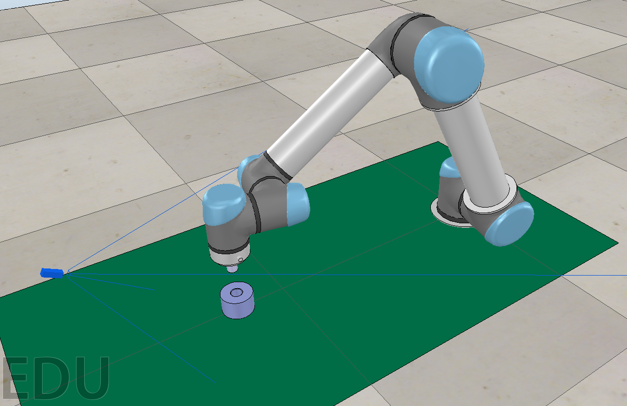
In this project, the UR5 manipulator is used in the simulation environment to insert the shaft at the end of the robot into the fixed hole, as shown in the following figure. Different from the direct assembly in the original paper, this scheme adopts two improvement measures:
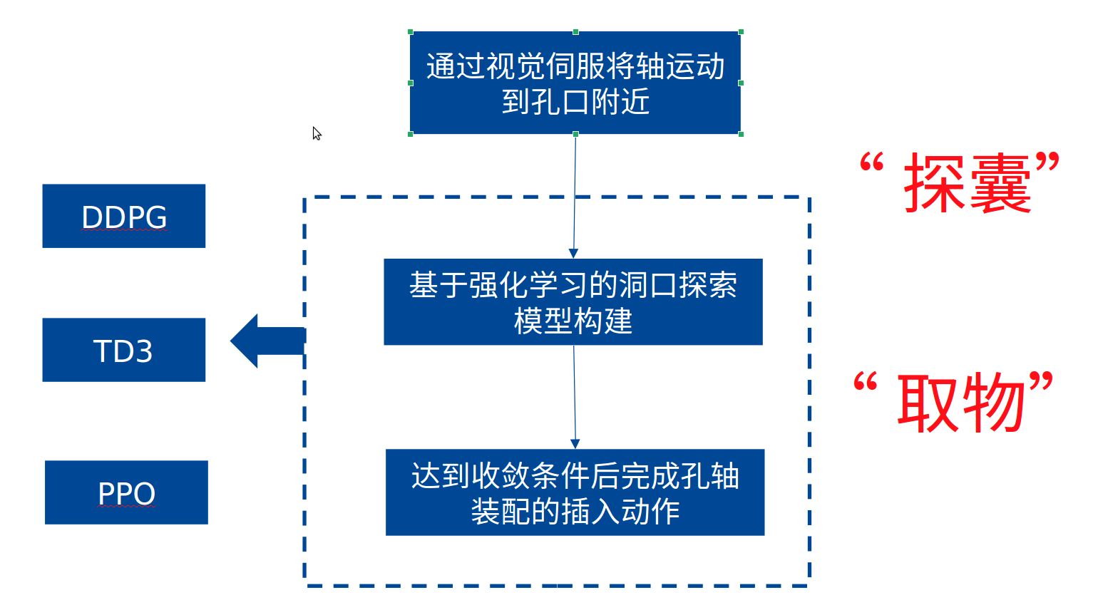
1) The initial position is changed to near the orifice (plus random disturbance), which can be realized by visual servo in engineering, and the technology is relatively mature
2) Change the jack scheme from "straight beating the Yellow Dragon" to "looking for things"

Combined with the problems existing in the original paper, the following improvement ideas are put forward

Problems in the original paper	Improvement ideas
Training time is too long (4 days and 4 nights)	Shorten step and episode
The training quality is poor and the success rate is low	Change the initial position so that it can obtain as much effective data as possible
Low learning efficiency	Reduce replay_buffer pool depth

system configuration

Coppelia Sim (V-REP simulation environment)

The environment used in this project is Ubuntu 16.04, and the version used is CoppeliaSim V4.2.0 rev5. For different systems, please select the corresponding version according to the options on the official website, CoppeliaSim Download After downloading, CoppeliaSim_Edu_V4_2_0_Ubuntu16_04 folder is the policy environment folder.

At coppeliasim_ Edu_ V4_ 2_ 0_ Ubuntu16_ Open the terminal under file 04 and enter. / coppeliaSim.sh.

 way@way:~/CoppeliaSim_Edu_V4_2_0_Ubuntu16_04$ ./coppeliaSim.sh

Creating a virtual environment using conda

tensorflow 1.14.0, 1.x and GPU Version (CUDA, cudnn) are used in this project. The graphics card is a GeForce GTX 1070/PCIe/SSE2. Here, Anaconda3 is recommended to create a virtual environment.
First, import the path of anaconda3. It is recommended to use the abbreviation in. bashrc and the corresponding environment in alias for easy operation:

alias condaenv="export PATH="/home/way/anaconda3/bin:$PATH""
alias condaact='source activate'
# To activate this environment, use
alias tf='conda activate tf114py36'
alias pytorch='conda activate pytorch'

Here tf is the environment we use. The creation method of conda is:
Create a new environment conda create -n tf114py36 python=3.6.0
Install tensorflow 1.14.0: CONDA install - n tf114py36 tensorflow GPU = = 1.14.0
Delete existing environment conda remove -n xxx
Switch environment conda activate xxx
Exit environment conda deactivate
View the installed package conda list

If all are installed, the steps to enter the environment are very simple. Three steps are OK: condaenv, condaact, tf

Program running

1. First run V-REP and open scene → \to → ur5_ force_ vision_ Insert-v0.ttt, import the hole axis model, and the size of the hole axis is shown in the figure below

FILE NAME	SHAPE	SIZE
peg0	circular	ϕ 20 × 30 \phi 20 \times 30 ϕ20×30
hole0	circular	ϕ 22 × 30 \phi22\times30 ϕ22×30
peg1	circular	ϕ 20 × 30 \phi 20 \times 30 ϕ20×30
hole1	circular	ϕ 23 × 30 \phi23\times30 ϕ23×30
peg2	square	20 × 20 × 30 20\times20\times30 20×20×30
hole2	square	23 × 23 × 30 23\times23\times30 23×23×30

1. Run the learning function in the tf environment. Take td3 as an example. python main_TD3.py

from vrepEnv import ArmEnv
import numpy as np
import os
from logger import Logger
import time
import datetime
import torch
import utils
import TD3



MAX_EPISODES = 10000
MAX_EP_STEPS = 10
ON_TRAIN = False //True if learning status
MEMORY_CAPACITY = 1000
BATCH_SIZE = 200
logging_directory = os.path.abspath('logs')
# logger = Logger(logging_directory)

# Set environment
env = ArmEnv()
state_dim = env.state_dim
action_dim = env.action_dim
a_bound = env.action_bound
seed = 0
torch.manual_seed(seed)
np.random.seed(seed)
pn = a_bound*0.2
nc = a_bound*0.5


# Set method: pd/RL

rl = TD3.TD3(state_dim, action_dim, a_bound,policy_noise=pn,noise_clip=nc)
replay_buffer = utils.ReplayBuffer(state_dim, action_dim,MEMORY_CAPACITY)

def train():
    """ Training the actor """

    logger = Logger(logging_directory)
    env.start_simulation()

    action_var = a_bound  # Action noise factor
    reward_value = []  # Record the reward value for each episode

    for episode in range(MAX_EPISODES):

        s = env.reset()
        episode_reward = 0.  # Total reward for an episode

        for step in range(MAX_EP_STEPS):
            print('step: %i '%(step))
            pn = action_var * 0.2
            nc = action_var * 0.5
            a = (
                    rl.select_action(np.array(s))
                    + np.random.normal(0, pn, size=action_dim)
            ).clip(-action_var, action_var)
            print('Action: ', a)

            #Perform action
            s_, r, done, safety = env.step(a)
            # Store data in replay buffer s, a, s_, r, done->not_done
            replay_buffer.add(s, a, s_, r, done)

            s = s_
            episode_reward += r
            mean_episode_reward = episode_reward/(step+1)

            if episode>MEMORY_CAPACITY:
                print('the memory is full')
                rl.train(replay_buffer,BATCH_SIZE)  # Start to learn once has fulfilled the memory
                action_var *= .999  # Reduce the action randomness once start to learn

            if done or step == MAX_EP_STEPS - 1 or safety == 1:
                print('Episode: %i | %s | %s | MER: %f | Steps: %i | Var: %f'
                      % (episode, 'Not inserted' if not done else 'Inserted', 'Unsafe' if safety == 1 else 'Safe',
                         mean_episode_reward, step, action_var))
                break

        reward_value.append(mean_episode_reward)

    logger.save_reward_value(reward_value)
    rl.save(logger.models_directory)

def test():
    models_directory = '/home/way/py/RL_UR_Project/UR5_RL_Assembly-inserted_discrete/logs/2020-12-21.22:51:59/models'
    rl.load(models_directory)
    s = env.reset()
    while True:
        a = rl.select_action(s)
        s, r, done, _ = env.step(a)
        if done and np.abs(s[12]) <= 10 and np.abs(s[13]) <= 10 and np.abs(s[14]) <= 10:
            env.move_to(np.array([s[0],s[1],0.011]),np.array([0, 0, 0]))
            time.sleep(3)
            break



if __name__ == '__main__':

    timestamp = time.time()
    timestamp_value = datetime.datetime.fromtimestamp(timestamp)
    print("The program starts at:  ", timestamp_value.strftime('%Y-%m-%d.%H:%M:%S'))

    if ON_TRAIN:
        train()
    else:
        test()

Comparison of experimental results

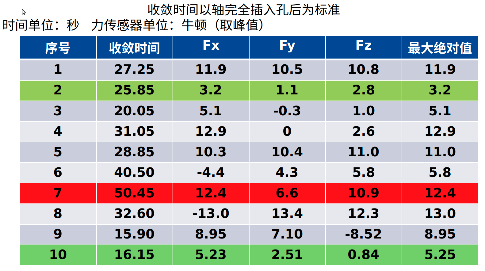
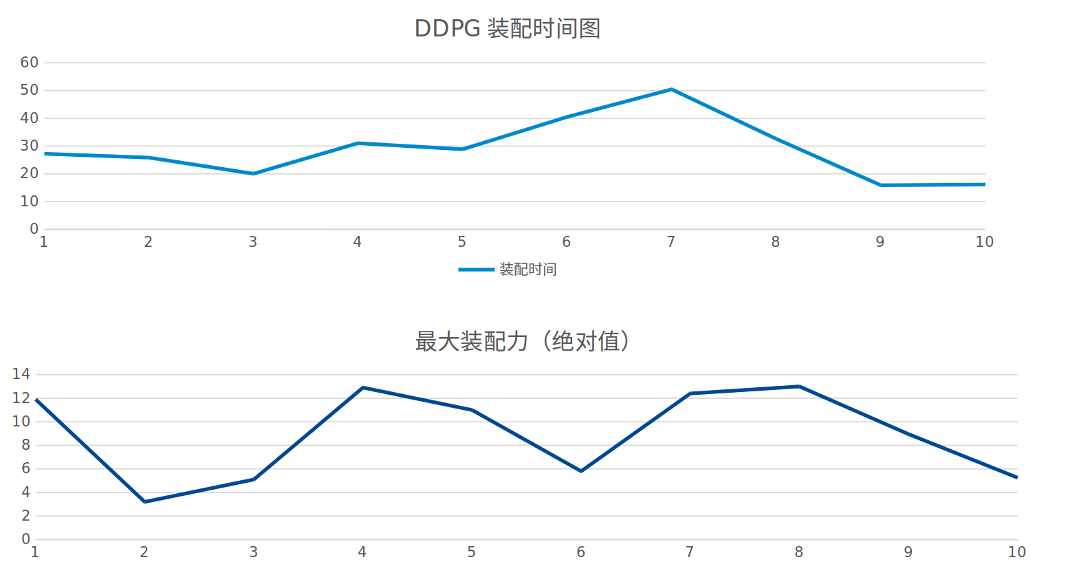
DDPG simulation effect

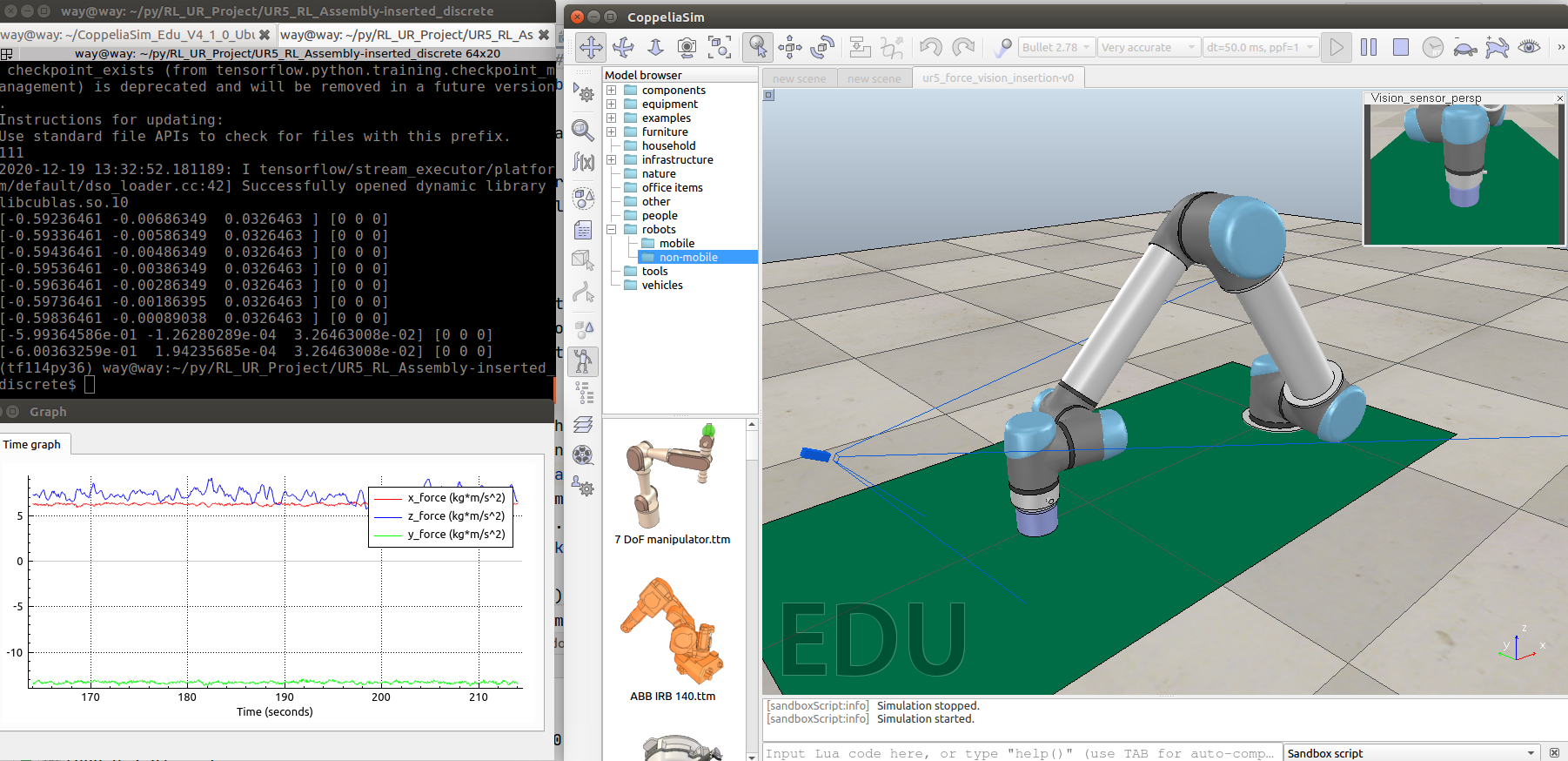
Effect picture of successful training

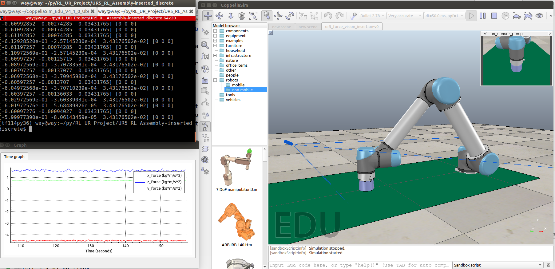
Effect drawing of training failure

Periodic oscillation occurs and it is difficult to converge

DDPG simulation results

Assembly time less than one minute, maximum assembly force less than 14 n, success rate: 85%

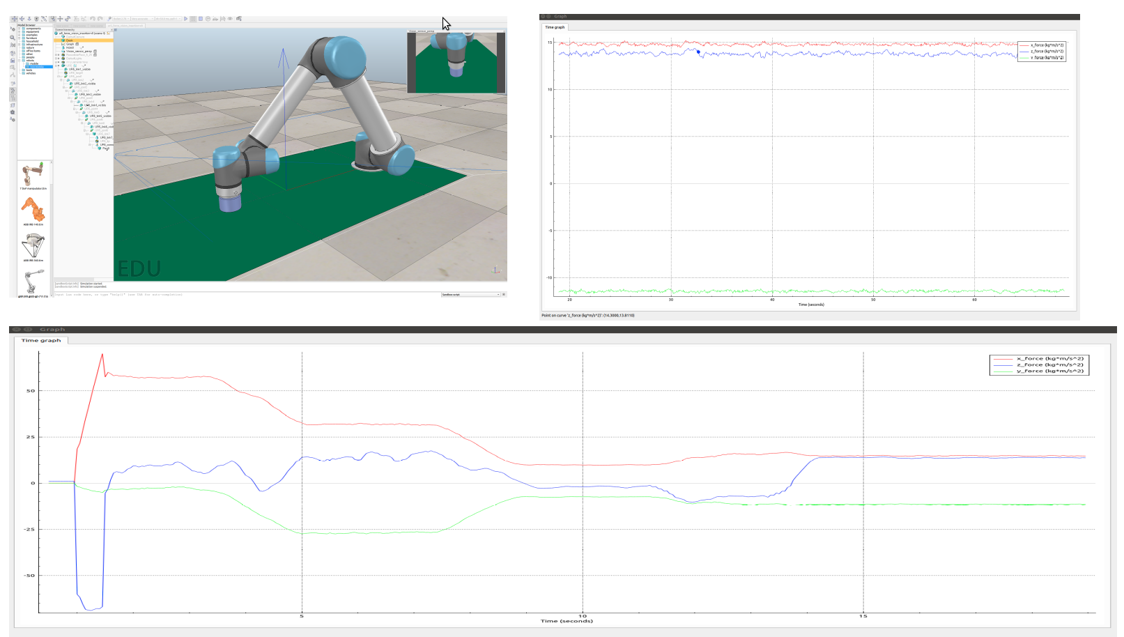
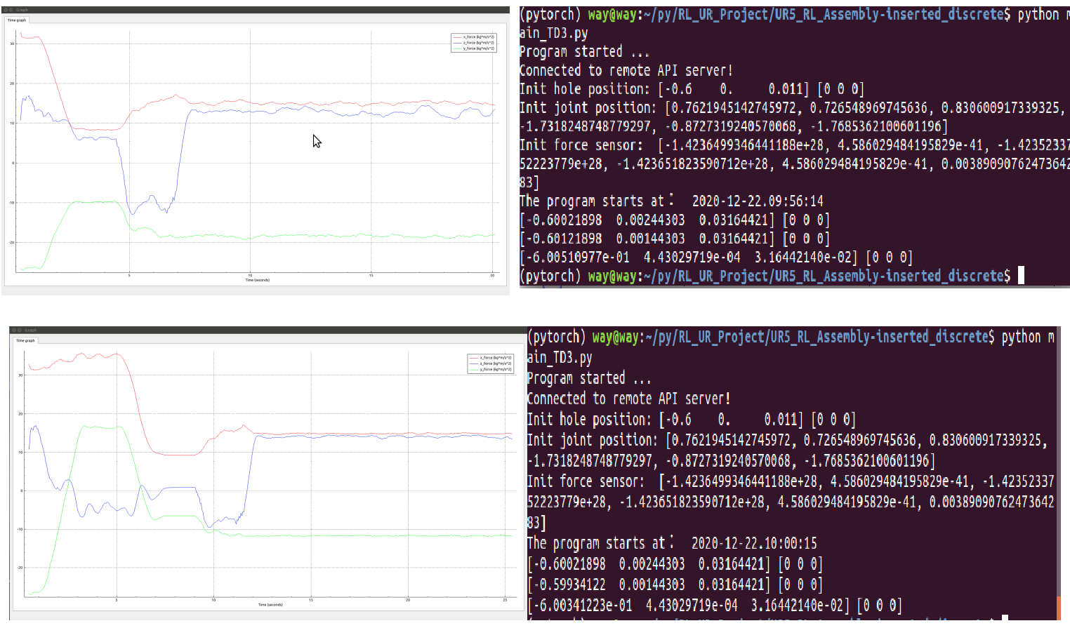
TD3 simulation effect

Effect picture of successful training

Training failure diagram

Final result divergence

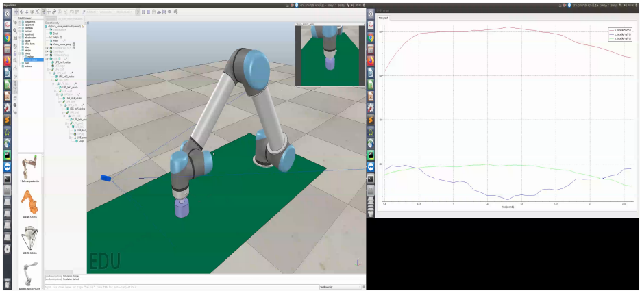
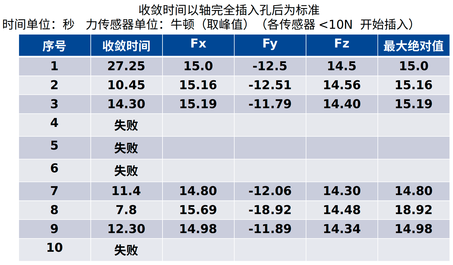
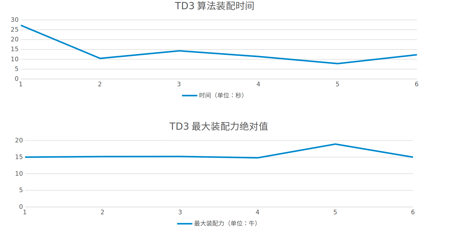
TD3 simulation results

The assembly time is less than 30 seconds, the maximum assembly force is less than 20 N, and the variance is small, the success rate is 60%

TD3 vs DDPG

project	TD3	DDPG
Success rate	60%	85%
Failure performance	Exponential divergence	Periodic oscillation is difficult to converge
Maximum assembly force	20 N	14 N
Average assembly time	15 s	30 s
Variance of assembly force	Small	large
Study time	one night	one night