1. Check the dataset for general information

import pandas as pd
fruits_df = pd.read_table('fruit_data_width_colors.txt')
print(fruits_df.head(10))
print('Number of samples:',len(fruits_df))

The output information is:

    fruit_label fruit_name     fruit_subtype  mass  width  height  color_score
0             1      apple      granny_smith   192    8.4     7.3         0.55
1             1      apple      granny_smith   180    8.0     6.8         0.59
2             1      apple      granny_smith   176    7.4     7.2         0.60
3             2   mandarin          mandarin    86    6.2     4.7         0.80
4             2   mandarin          mandarin    84    6.0     4.6         0.79
5             2   mandarin          mandarin    80    5.8     4.3         0.77
6             2   mandarin          mandarin    80    5.9     4.3         0.81
7             2   mandarin          mandarin    76    5.8     4.0         0.81
8             1      apple          braeburn   178    7.1     7.8         0.92
9             1      apple          braeburn   172    7.4     7.0         0.89
 Number of samples: 59

We can observe that the data are fruit label, fruit name, fruit type, fruit quality, width, height and color score

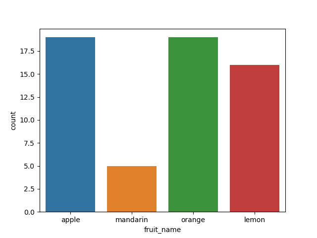
We continue to understand the sample size of each fruit by drawing

import seaborn as sns
sns.countplot(fruits_df['fruit_name'],label="Count")
plt.show()

The data volume of each fruit can be drawn

image.png

2. Data preprocessing

In the preprocessing stage, we need to divide the data into training data set and test data set. At the same time, in order to facilitate the comparison of predicted labels and real labels, we need to pair the fruit labels with the fruit names.

from sklearn.model_selection import train_test_split
#Tag pairing
fruit_name_dict = dict(zip(fruits_df['fruit_label'],fruits_df['fruit_name']))
print(fruit_name_dict)
#Divide training set and test set
X = fruits_df[['mass','width','height','color_score']]
y = fruits_df['fruit_label']

X_train,X_test,y_train,y_test = train_test_split(X,y,test_size=1/4,random_state=0)
print('Number of dataset samples:{},Number of training samples:{},Number of test set samples:{}'.format(len(X),len(X_train),len(X_test)))

Return output result:

{1: 'apple', 2: 'mandarin', 3: 'orange', 4: 'lemon'}
Number of data set samples: 59,Number of training samples: 44,Number of test set samples: 15

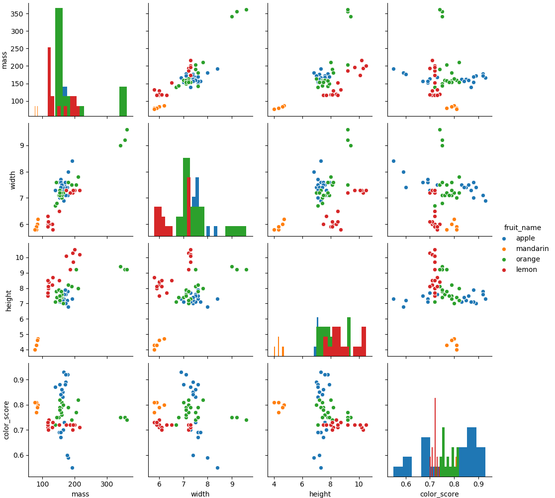
Here, we can also visualize the variable relationship to pave the way for the next step:

sns.pairplot(data=fruits_df,hue='fruit_name',vars=['mass','width','height','color_score'],diag_kind='hist')
plt.show()

You can draw the relationship between various variables

image.png

3. Establish model and training model

We use the kNN nearest neighbor algorithm model in sklearn. The k-nearest neighbor algorithm is a sample based algorithm (nonparametric model). The steps of the algorithm are as follows:

1. Calculate the distance between the test sample and all training samples
2. Select k training samples with the smallest distance from them for the test samples
3. The classification to which most of the k training samples belong is counted
4. This classification is the classification to which the data to be classified belongs

For this algorithm model, we need to artificially give a k value, that is, judge through several nearest data points. This can be judged according to the visual graphics we have made before. How to get the optimal number of adjacent points?
We can use cross validation

On the one hand, we can determine it through visual graphics. On the other hand, we can try several more k values to see the prediction accuracy

Let's first set the k value to 5

from sklearn.neighbors import KNeighborsClassifier
knn = KNeighborsClassifier(n_neighbors=5) #Model building
knn.fit(X_train,y_train) #Training model

Let's test the model:

from sklearn.metrics import accuracy_score
y_pred = knn.predict(X_test)
print('Forecast tab:'，y_pred)
print('True label:', y_test.values)
acc = accurancy_score(y_test,y_pred)
print('Accuracy:',acc)

Output results:

Forecast tab: [3 1 4 4 1 1 3 3 1 4 2 1 3 1 4]
True label: [3 3 4 3 1 1 3 4 3 1 2 1 3 3 3]
Accuracy: 0.5333333333333333

4. Adjust the model

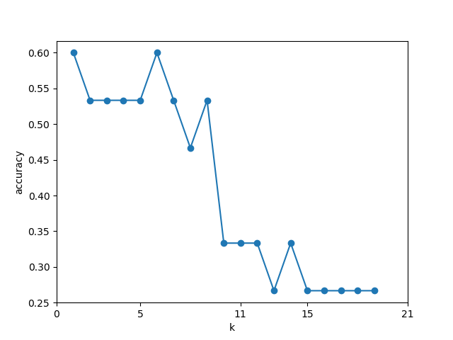
Let's test the test accuracy corresponding to each k value to see how high the accuracy is when the K value is taken:

k_range = range(1,20)
acc_scores = []

for k in k_range:
    knn = KNeighborsClassifier(n_neighbors=k)
    knn.fit(X_train,y_train)
    acc_scores.append((knn.score(X_test,y_test)))

plt.figure()
plt.xlabel('k')
plt.ylabel('accuracy')
plt.plot(k_range,acc_scores,marker='o')
plt.xticks([0,5,11,15,21])
plt.show()

The returned picture is:

image.png

It can be seen that when the value of k is 6, the accuracy is the highest, which is 0.6

Through this practice, we can understand the k-nearest neighbor algorithm
Problems needing attention:

1. Similarity measure
2. Number of nearest neighbor points, and the optimal number of nearest neighbor points is obtained through cross validation

Advantages and disadvantages of kNN:
Advantages: the algorithm is simple and intuitive, easy to implement, does not need additional data, and only depends on the data itself
Disadvantages: large amount of calculation, slow classification speed, and k value needs to be specified in advance

Data file and code (Baidu network disk)
Extraction code: br30