I. First Identity HMM

Hidden Markov Model (HMM) is a statistical model used to describe the hidden unknown parameters. HMM has been successfully used in speech recognition, text classification, bioinformatics, fault diagnosis and life prediction.

HMM can be composed of three elements:= (A,B,II), where A is the state transition probability matrix, B is the observed state probability matrix, and II is the hidden state initial probability distribution.

HMM has two basic assumptions, one is the Homogeneous Markov hypothesis, the state of hidden Markov chain t is only related to the t-1 state, the other is the observation independence hypothesis, and the observation is only related to the current state at the moment.

HMM solves three issues:

• The first is the probability calculation problem, known models and observation series, which calculates the probability of occurrence of observation series. The method to solve this problem is forward-backward method.

• The second is the learning problem, known observation sequence, estimating model parameters, which is solved by the Baum-Welch algorithm

• The third is the prediction problem (decoding problem), the known model and observation sequence, and the solution of the state sequence, which is solved by the dynamic programming Viterbi algorithm.

HMM implementation: python's hmmlearn s can be divided into two categories according to whether the observation state is continuous or discrete. GaussianHMM and GMMHMM are HMM models of continuous observation state; MultinomialHMM is a model of discrete observation state.

2. Example Analysis

(1) Description of the problem: stock forecast problem, the observed value is the rise of the stock (closing price on the day - closing price on the previous day) and the volume of trading. The hidden state is assumed to be flat, falling and rising. HMM is constructed based on the historical data of the stock, and the closing price of the stock is further predicted.

(2) Data preprocessing: extract useful columns from the original data, and do outlier processing operations to get the data data of the model, the original data is a stock 2013-2019 record data, as shown in the following figure.

import datetime
import numpy as np
import pandas as pd
from matplotlib import cm, pyplot as plt
from hmmlearn.hmm import GaussianHMM
#data processing
df = pd.read_excel("601668.SH.xlsx", header=0)
print("Size of original data:", df.shape)
print("Column name of original data", df.columns)
df['date'] = pd.to_datetime(df['date'])
df.reset_index(inplace=True, drop=False)
df.drop(['index','Transaction Date','Opening price','Top Price','Minimum price' ,'market value', 'Turnover rate', 'pe', 'pb'], axis=1, inplace=True)
df['date'] = df['date'].apply(datetime.datetime.toordinal)
print(df.head())
dates = df['date'][1:]
close_v = df['Closing price']
volume = df['volume'][1:]
diff = np.diff(close_v)
#Get Input Data
X = np.column_stack([diff, volume])
print("Size of input data:", X.shape)   #(1504, 2)

(3) Handling of outliers:

min = X.mean(axis=0)[0] - 8*X.std(axis=0)[0]   #minimum value
max = X.mean(axis=0)[0] + 8*X.std(axis=0)[0]  #Maximum
X = pd.DataFrame(X)
#Set outlier to mean
for i in range(len(X)):  #Traversal of dataframe
    if (X.loc[i, 0]< min) | (X.loc[i, 0] > max):
            X.loc[i, 0] = X.mean(axis=0)[0]

(4) Model building:

#Partition of datasets
X_Test = X.iloc[:-30]
X_Pre = X.iloc[-30:]
print("Size of training set:", X_Test.shape)     #(1474, 2)
print("Test Set Size:", X_Pre.shape)      #(30, 2)
#Modeling
model = GaussianHMM(n_components=3, covariance_type='diag', n_iter=1000) 
model.fit(X_Test)
print("Number of hidden states", model.n_components)  #
print("Mean Matrix")
print(model.means_)
print("covariance matrix")
print(model.covars_)
print("State Transition Matrix--A")
print(model.transmat_)

 

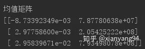
Mean Matrix: There are three rows, each representing a hidden layer state (state 0, 1, 2), and each row's two elements representing the mean of the rise and the mean of the volume. Since the change in the stock is not particularly large, the result is not particularly obvious, but a negative state 0 mean can be observed, which can be interpreted as a "fall"The mean of state 1 is the smallest, close to 0, which can be interpreted as "flat", the mean of state 2 is positive, and can be interpreted as "rise".

 

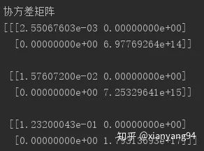
Covariance Matrix: There are three covariance matrices corresponding to three hidden layer states. The diagonal value is the variance of the state, the larger the variance, the less trustworthy the prediction representing the state. The variance of state 0 is about 0.00255, the variance of state 0 is the smallest, the prediction is very trustworthy; the variance of state 1 is about 0.0157, the confidence is intermediate; the variance of state 2 is 0.1232, the variance of state 2 is the largest and the most untrustworthy.

State Transition Matrix: The transition probability representing the state of three hidden layers. It can be seen that the diagonal value is larger, that is, state 0, 1, 2 tend to maintain the current state, which means the stock is more stable.

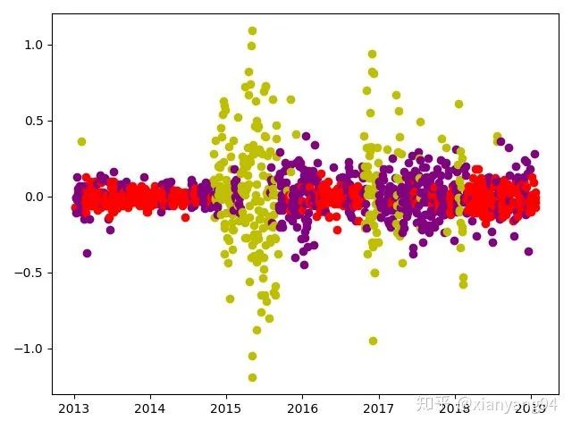
(5) Hidden state partition results:

#Hidden state partition of training data
X_pic = np.column_stack([dates[:-30], hidden_states, X_Test])
for i in range(len(X_pic)):
    if X_pic[i, 1] == 0:
        plt.plot_date(x=X_pic[i, 0],y=X_pic[i,2],color='r')
    elif X_pic[i, 1] == 1:
        plt.plot_date(x=X_pic[i, 0],y=X_pic[i,2],color='purple')
    else:plt.plot_date(x=X_pic[i, 0],y=X_pic[i,2],color ='y')
plt.show()

 

(6) Prediction value calculation:

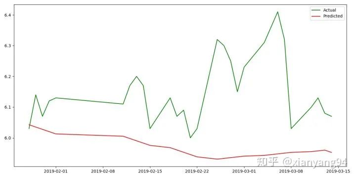
The first set of forecast data is used as the initial data to predict the stock's rise in the next period, and so on to predict the price of the last 30 groups of the stock.

expected_returns_volumes = np.dot(model.transmat_, model.means_)
expected_returns = expected_returns_volumes[:,0]        
predicted_price = []  #predicted value
current_price = close_v.iloc[-30]
for i in range(len(X_Pre)):
    hidden_states = model.predict(X_Pre.iloc[i].values.reshape(1,2))  #Use the first set of predictions as initial values
    predicted_price.append(current_price+expected_returns[hidden_states])
    current_price = predicted_price[i]

 

3. Summary

It can be seen that the trend of the predicted result is consistent with the true value, but the predicted result is not good. The accuracy of the prediction can be improved by increasing the amount of training data and adjusting the model parameters. HMM application scenario: the research problem is sequence-based, such as time series or state series; there are two states of significance, one is the observation sequence, the other is the hidden state sequence.Compared with the RNN, LSTM and other neural network sequence models, HMM predicts poorly. In summary, the stock market is risky and investment needs to be careful.

Reference: official hmmlearn document

https://hmmlearn.readthedocs.io/en/latest/

Use Hidden Markov Model to Predict Stock Price Trend_Python Chinese Community-CSDN Blog