Competition background
Based on the analysis of network public opinion, the competition questions require players to conduct data analysis and visualization of brand issues according to users' comments. Through this competition question, we can guide the commonly used data visualization charts and data analysis methods to conduct exploratory data analysis on the content of interest.
Competition data
Data source: earphone_sentiment.csv, for 10000 + industry users' comments on headphones
Using Tianchi lab to play games, you can mount the data source directly in the notebook
https://tianchi.aliyun.com/competition/entrance/531890/information
Competition task
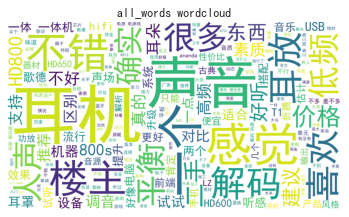
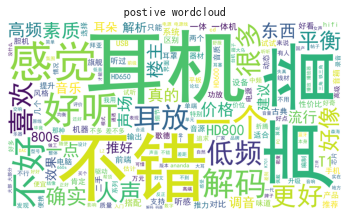
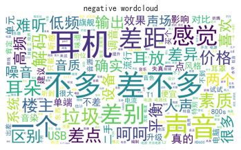
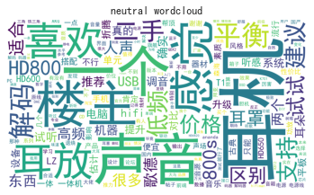
1) Word cloud visualization (keywords in comments, word clouds with different emotions)
2) Histogram (different topics, different emotions, different emotional words)
3) Correlation coefficient heat map (different topics, different emotions, different emotional words)
To use python as a word cloud, you need to install two packages: Chinese word segmentation jieba and wordcloud
1 data exploration
#Import package
import pandas as pd
import numpy as np
import jieba
import sys
from wordcloud import WordCloud,STOPWORDS
from imageio import imread
import matplotlib.pyplot as plt
import seaborn as sns
from collections import Counter
from pylab import *
plt.rcParams['font.sans-serif']=['SimHei']
plt.rcParams['axes.unicode_minus']=False

sns.set_style('darkgrid',{'font.sans-serif':['SimHei','DejaVa Sans']})
#Import data
earphone_sentiment=pd.read_csv('./earphone_sentiment.csv')
earphone_sentiment
1.1 check the data type and detect duplicate and missing values
#View duplicate values
print(earphone_sentiment.duplicated().sum())
#View missing values for fields
print(earphone_sentiment.isnull().sum())
# View data fields, non null values, data types, etc
earphone_sentiment.info()
No duplicate rows were found in the dataset, where sentiment_ Only 4966 of the word column is non empty and has a large number of empty values of 12210. It is necessary to investigate whether the empty value needs to be handled.
The dataset has 17176 rows of records and 5 fields in total.
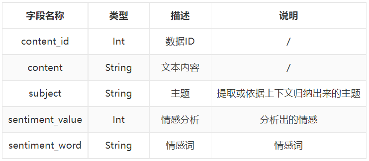
0 content_id (int64): data id
1. Content (object): text content
2 subject (object): subject
3 sentiment_word (object): emotional word
4 sentiment_value (int64): emotional tendency analysis
#Perspective the emotional words of different themes with different emotional tendencies and view the data
earphone_sentiment.pivot_table(columns='sentiment_value',index='subject',values='sentiment_word',aggfunc="count")
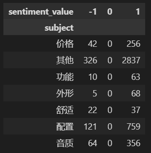
You can see from the perspective data:
1. The values of emotional tendency are: - 1 (negative emotion), 0 (neutral emotion) and 1 (positive emotion)
2. There are 7 themes in total: price, function, appearance, comfort, configuration, sound quality and others
3,‘sentiment_ All null values in the 'word' column belong to neutral emotional tendency (0), and there are no emotional words, so they are not processed.
1.2 data preprocessing
Call out the disabled Dictionary (you need to eliminate some meaningless words, such as De, Di, De, do, feel, headset, ha ha, hee hee, Zai, and some punctuation marks; the dictionary can be found on the Internet or established by yourself
#Read inactive dictionary
stop_words=[]
with open(r'./chineseStopWords.txt','r') as f:
    for line in f:
        stop_words.append(line.strip('\n').split(',')[0])
#participle
df=earphone_sentiment.copy()

row,col=df.shape  #Number of rows in the data table
df['cutwords'] = 'cutwords'  #Predefined list

for i in np.arange(row):
    cutword = [x for x in jieba.cut_for_search(df.content[i]) if len(x) > 1]  #Segment words and remove words of length 1
    cutword = [k for k in cutword if k not in stop_words]  #Remove stop words
    df.cutwords[i]=cutword

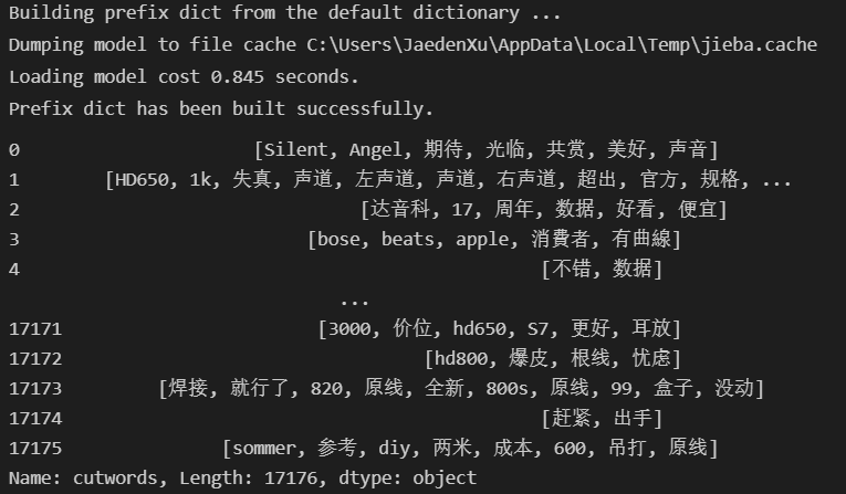
#View all word segmentation results
df.cutwords
#Assign emotion analysis score to Chinese
new_value={-1:"negative",0:"neutral",1:"positive"}
df['sentiment_value']=df['sentiment_value'].map(new_value)

#Screening data on positive emotional tendencies
pos_df=df.loc[df['sentiment_value']=='positive']
#Screening data on positive emotional tendencies
neg_df=df.loc[df['sentiment_value']=='negative']
#Screening data on neutral emotional tendencies
neu_df=df.loc[df['sentiment_value']=='neutral']
2. User emotion visualization
2.1 task 1: word cloud visualization
(keywords in comments, word clouds with different emotions)
#Join all participles
all_text='/'.join(np.concatenate(df.cutwords))

#Participle linking positive emotions
positive_text='/'.join(np.concatenate(pos_df.cutwords.reset_index(drop=True)))

#Participle linking negative emotions
negative_text='/'.join(np.concatenate(neg_df.cutwords.reset_index(drop=True)))

#Participle linking neutral emotions
neutral_text='/'.join(np.concatenate(neu_df.cutwords.reset_index(drop=True)))

#Import word cloud basemap
earphone_mark=imread(r'./cloud.png')
pos_mark=imread(r'./cloud.png')
neu_mark=imread(r'./cloud.png')
neg_mark=imread(r'./cloud.png')
#Drawing word cloud using text

#Draw total word cloud
wc1=WordCloud(font_path='simhei.ttf',background_color='white',margin=5,width=1800,height=800,mask=earphone_mark).generate(all_text)
plt.imshow(wc1)
plt.axis("off")
plt.title('all_words wordcloud')
plt.show()

#Draw words for positive emotions
wc2=WordCloud(font_path='simhei.ttf',background_color='white',margin=5,width=1800,height=800,mask=pos_mark).generate(positive_text)
plt.imshow(wc2)
plt.axis("off")
plt.title('postive wordcloud')
plt.show()

#Draw negative emotional words
wc3=WordCloud(font_path='simhei.ttf',background_color='white',margin=5,width=1800,height=800,mask=neg_mark).generate(negative_text)
plt.imshow(wc3)
plt.axis("off")
plt.title('negative wordcloud')
plt.show()

#Draw neutral emotional words
wc3=WordCloud(font_path='simhei.ttf',background_color='white',margin=5,width=1800,height=800,mask=neu_mark).generate(neutral_text)
plt.imshow(wc3)
plt.axis("off")
plt.title('neutral wordcloud')
plt.show()
2.2 task 2: histogram
(different themes, different emotions, different emotional words)
2.2.1 histogram of emotional words with different emotional tendencies and different topics
#Those with neutral emotional tendency have no emotional words and are excluded
df_vsw=df.loc[df['sentiment_value']!='neutral'].pivot_table(columns='sentiment_value',index='subject',values='sentiment_word',aggfunc="count")
print(df_vsw)

#Draw histogram
plt.figure(figsize=(20,15))
df_vsw.plot.bar()

#Mark label (ha is the position)

for x,y in enumerate(df_vsw['negative'].values):
    plt.text(x,y,"%s" %y,ha='right')
for x,y in enumerate(df_vsw['positive'].values):
    plt.text(x,y,"%s" %y,ha='left')

plt.ylabel('number of sentiment_word')
plt.title('Number of emotional words with different emotional tendencies and themes')
plt.show()
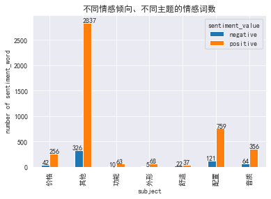
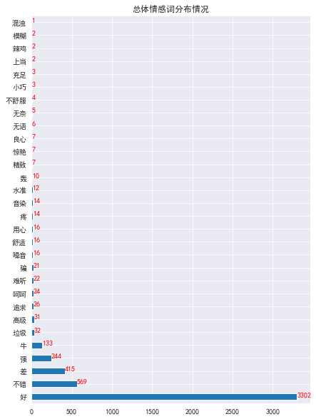
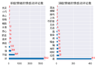
2.2.2 number of emotional word comments with different emotional tendencies - horizontal histogram
#Number of comments on different emotional words with different emotional tendencies
df2=df['sentiment_word'].value_counts()

#Number of emotional word comments of positive emotion
df2_pos=pos_df.sentiment_word.value_counts()

#Number of emotional word reviews of negative emotions
df2_neg=neg_df.sentiment_word.value_counts()
#Overall distribution of emotional words
plt.figure(figsize=(7,10))
df2.plot.barh()
for y,x in enumerate(df2.values):
    plt.text(x,y,"%s" %x,color='red')
plt.title('Overall emotional word distribution')
plt.show()


#Distribution of emotional words with different emotional tendencies
plt.subplot(1,2,1)
df2_pos.plot.barh()
for y,x in enumerate(df2_pos.values):
    plt.text(x,y,"%s" %x,color='red')
plt.title('Number of emotional word comments of positive emotion')

plt.subplot(1,2,2)
df2_neg.plot.barh()
for y,x in enumerate(df2_neg.values):
    plt.text(x,y,"%s" %x,color='red')
plt.title('Number of emotional word reviews of negative emotions')
plt.subplots_adjust(wspace=0.3) #Adjust the horizontal distance between the two figures
plt.show()
2.3 task 3: correlation coefficient thermodynamic diagram
(different themes, different emotions, different emotional words)
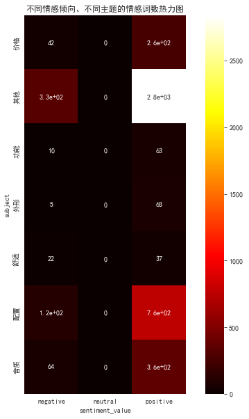
2.3.1 number of emotional words with different emotional tendencies and themes - correlation heat map
df_vsw=df.pivot_table(columns='sentiment_value',index='subject',values='sentiment_word',aggfunc="count")

plt.figure(figsize=(10,10))
with sns.axes_style("white"):
    ax=sns.heatmap(df_vsw,square=True,annot=True,cmap='hot')
ax.set_title("Heat map of emotional words with different emotional tendencies and different topics")
plt.show()
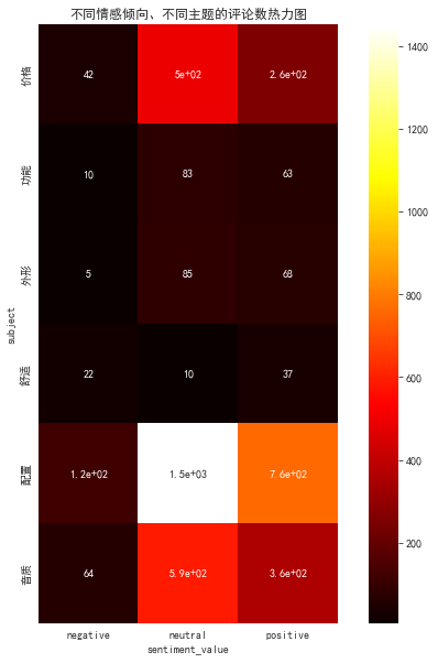
2.3.2 number of comments with different emotional tendencies and different topics - correlation heat map
df_vsc=df.pivot_table(columns='sentiment_value',index='subject',values='content',aggfunc="count")
print(df_vsc)
#Because "other" topics have relatively little analysis significance, and the number is too large, which will affect the effect of thermal diagram, the analysis is excluded
df_vsc1=df_vsc.drop("other")

plt.figure(figsize=(10,10))
with sns.axes_style("white"):
    ax=sns.heatmap(df_vsc1,square=True,annot=True,cmap='hot')
ax.set_title("Heat map of comments on different emotional tendencies and different topics")
plt.show()
