Spatial object data visualization

In the process of spatial data processing and analysis, a main feature is to visualize spatial objects and make exquisite maps. This section introduces the method of spatial visualization.

• Load packages and data

Spatial data visualization 
#example 
library(maptools) 
require(rgeos) 
LN.bou <- readShapePoly("LondonBorough",verbose = T,proj4string = CRS("+init=epsg:27700")) 

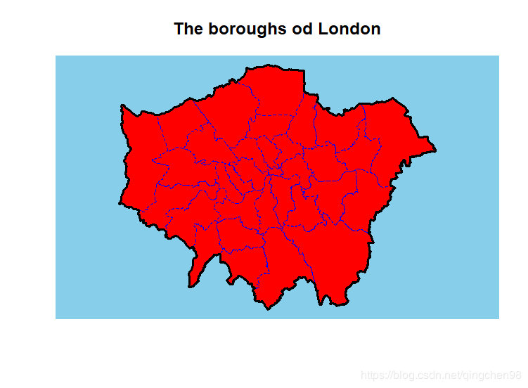
• By making a separate administrative boundary of London, it is superimposed with the original London brough data, and the color scheme and contour width are modified

#Fusion boundary 
LN.outline <- gUnaryUnion(LN.bou,id=NULL) 
#Color scheme settings 
plot(LN.bou,col="red",bg="skyblue",lty=2,border="blue") 
#Overlay boundary layer 
plot(LN.outline,lwd=3,add=T) 
#Add title 
title(main = "The boroughs od London",font.main=2,cex.main=1.5)

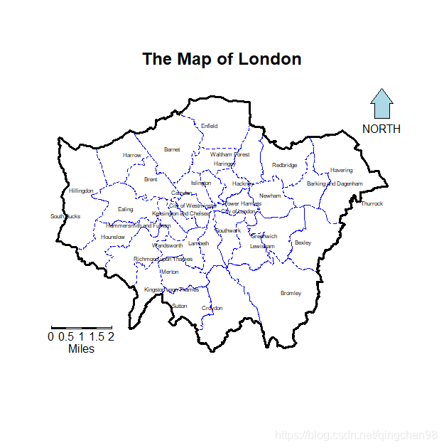
• The functions pointLabel, mapscale and North are provided in the function package maptools Arrow, which is used to add text annotation, scale bar and compass respectively in the drawing. The following code can add corresponding drawing elements in the previous drawing

##Add drawing element 
library(maptools)
library(GISTools) 
plot(LN.bou,col="white",lty=2,border="blue") 
plot(LN.outline,lwd=3,add=T) 
coords <- coordinates(LN.bou) pointLabel(coords[,1],coords[,2],LN.bou@data[,"NAME"],doPlot = T,cex = 0.5) 
map.scale(511000,159850,miles2ft(2),"Miles",4,0.5) north.arrow(561000,197000,miles2ft(0.25),col="lightblue") 
title(main = "The Map of London",font.main=2,cex.main=1.5)

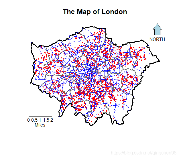
• Overlay and display layers and make personalized maps

#Load London house price data and road network data 
LNNTa <- readShapeLines("LNNTa",verbose = TRUE,proj4string = CRS("+init=epsg:27700")) 
LNHP <- readShapePoints("LNHP",verbose = TRUE,proj4string = CRS("+init=epsg:27700")) 
#Overlay and display the administrative division data, road network data and house price data of London, and make a personalized map plot(LN.bou,col="white",lty=1,lwd=2,border="grey40") 
plot(LN.outline,lwd=3,add=T) 
plot(LNHP,pch=16,col="red",cex=0.5,add=T) 
plot(LNNTa,col="blue",lty=2,lwd=1.5,add=T)
map.scale(508000,159850,miles2ft(2),"Miles",4,0.5)
north.arrow(561000,197000,miles2ft(0.25),col="lightblue") 
title(main = "The Map of London",font.main=2,cex.main=1.5)

• Grid data visualization

Grid data visualization
library(raster)
LN.lat <- raster(nrow=30,ncol=60,ex=extent(LN.bou))
LN.lat <- rasterize(LN.bou,LN.lat,"NAME")
LN.gr <- as(LN.lat,"SpatialGridDataFrame")
LN.p <- as(LN.lat,"SpatialPixelsDataFrame")
image(LN.gr,col=brewer.pal(7,"YlOrRd"))
map.scale(508000,159850,miles2ft(2),"Miles",4,0.5)
north.arrow(561000,197000,miles2ft(0.25),col="lightblue")
title(main = "Grid data visualization example",font.main=2,cex.main=1.5)

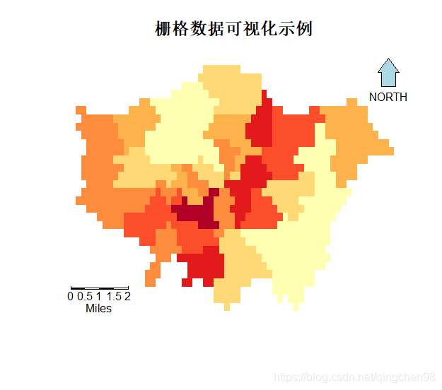
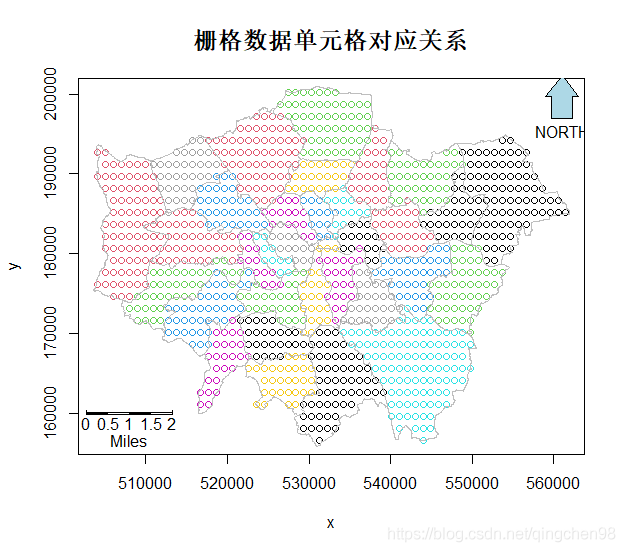
The corresponding relationship of grid data units is as follows:

Visualization of spatial attribute data

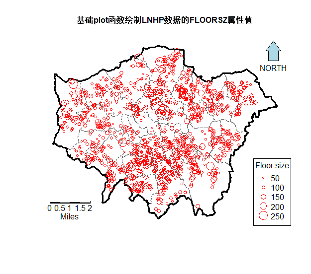
• According to the FLOORSZ attribute (house area) in London house price data LNHP, the corresponding area size is expressed by the size of the point, and the point sizes representing 50, 100, 150, 200 and 250 square meters are marked and explained by using the legend function.

####Visualization of spatial attribute data
#Draws the FLOORSZ attribute value of LNHP data
plot(LN.bou,col="white",lty=2,lwd=1,border="grey40")
plot(LN.outline,lwd=3,add=T)
plot(LNHP,pch=1,col="red",cex=LNHP@data$FLOORSZ/100,add=T)
legVals <- c(50,100,150,200,250)
legend("bottomright",legend = legVals,pch = 1,col = "red",
       pt.cex = legVals/100,title = "Floor size")
map.scale(508000,159850,miles2ft(2),"Miles",4,0.5)
north.arrow(561000,197000,miles2ft(0.25),col="lightblue")
title(main = "Basics plot Function drawing LNHP Data FLOORSZ Attribute value",font.main=2,cex.main=1)

• The function package sp provides a visual function spplot, which uses color to distinguish the spatial attribute values of different intervals

#Rsln ssplot data value of HP function rslnssplot
library(sp)
mypalette <- brewer.pal(6,"Reds")
spplot(LNHP,"FLOORSZ",key.space="right",pch=16,cex=LNHP$FLOORSZ/100,
       col.regions=mypalette,cuts=6)

• When assigning multiple attributes at the same time, the function spot can automatically draw the corresponding attribute items in the same drawing medium object. As shown in the figure, different house type attributes ("TYPEDETCH", "tpsemitch", "TYPEBNGLW", "TYPETRRD") are drawn. Each attribute value is 0 or 1, and 1 represents that the current data point is the house of the corresponding type

##The spot function plots multiple attribute values of LNHP data at the same time
mypalette <- brewer.pal(3,"Reds")
spplot(LNHP,c("TYPEDETCH","TPSEMIDTCH","TYPEBNGLW","TYPETRRD"),key.space="right",pch=16,
       col.regions=mypalette,cex=0.5,cuts=2)

• When using the function spplot to draw a thematic map, you can add mapping elements such as compass, scale bar and other layer elements to be displayed through sp.layout

#Add drawing features with the parameter sp.layout
mypalette <- brewer.pal(6,"YlOrRd")
map.na <- list("SpatialPolygonsRescale",layout.north.arrow(),offset = c(556000,195000),
               scale = 4000, col=1)
map.scale.1 <- list("SpatialPolygonsRescale",layout.scale.bar(),offset = c(511000,158000),
                    scale=5000,col=1,fill=c("transparent","green"))
map.scale.2 <- list("sp.text",c(511000,157000),"0",cex=0.8,col=1)
map.scale.3 <- list("sp.text",c(517000,157000),"5km",cex=0.9,col=1)
LN_bou <- list("sp.polygons",LN.bou)
map.layout <- list(LN_bou,map.na,map.scale.1,map.scale.2,map.scale.3)
spplot(LNHP,"FLOORSZ",key.space="right",pch=16,col.regions=mypalette,cuts=6,sp.layout=map.layout)

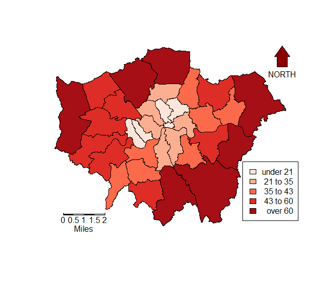
• In the function package GISTools, the function choropleth is provided, which is specially used for the thematic map making of polygon data objects, combined with auto The shading function is used to define the interval division of the value range and the corresponding color, choro The legend function is used to draw the corresponding legend

#Making thematic map with choropleth function
library(rgeos)
LN.bou$AREA <- gArea(LN.bou,byid = T)/(1e+6)
shades <- auto.shading(LN.bou$AREA)
choropleth(LN.bou,LN.bou$AREA)
choro.legend(551000,172000,shades)
map.scale(511000,158550,miles2ft(2),"Miles",4,0.5)
north.arrow(561000,196000,miles2ft(0.25),col="darkred")