Absrtact: linear programming is a set of mathematical and computational tools that enable you to find a specific solution of the system, which corresponds to the maximum or minimum of some other linear functions.

This article is shared from Huawei cloud community< Practicing linear programming: optimizing with Python >, author: Yuchuan.

Description of linear programming

What is linear programming?

Imagine that you have a system of linear equations and inequalities. Such systems usually have many possible solutions. Linear programming is a set of mathematical and computational tools that allows you to find a specific solution of the system that corresponds to the maximum or minimum of some other linear function.

What is mixed integer linear programming?

Mixed integer linear programming is an extension of linear programming. It deals with the problem that at least one variable adopts discrete integers instead of continuous values. Although at first glance, mixed integer problems are similar to continuous variable problems, they have significant advantages in flexibility and accuracy.

Integer variables are important to correctly represent the number of natural integers, such as the number of aircraft produced or the number of customers served.

A particularly important integer variable is a binary variable. It can only take a value of zero or one and is useful in making a yes or no decision, such as whether a factory should be built or whether machines should be turned on or off. You can also use them to simulate logical constraints.

Why is linear programming important?

Linear programming is a basic optimization technology, which has been used in science and mathematics intensive fields for decades. It is accurate, relatively fast and suitable for a series of practical applications.

Mixed integer linear programming allows you to overcome many limitations of linear programming. You can use piecewise linear functions to approximate nonlinear functions, semi continuous variables, model logic constraints, and so on. It is a computationally intensive tool, but advances in computer hardware and software make it more applicable every day.

Usually, when people try to formulate and solve optimization problems, the first problem is whether they can apply linear programming or mixed integer linear programming.

The following article illustrates some use cases of linear programming and mixed integer linear programming:

• Gurobi optimization case study
• Five application fields of linear programming technology

With the enhancement of computer ability, the improvement of algorithms and the emergence of more user-friendly software solutions, the importance of linear programming, especially mixed integer linear programming, increases with the passage of time.

Linear programming using Python

The basic method to solve linear programming problems is called simplex method, which has many variants. Another popular method is the interior point method.

The mixed integer linear programming problem can be solved by more complex and more computational methods, such as branch and bound method, which uses linear programming behind the scenes. Some variations of this method are the branching and cutting method, which involves the use of cutting planes, as well as the branching and price method.

There are several suitable and well-known Python tools for linear programming and mixed integer linear programming. Some of them are open source, while others are proprietary. Whether you need free or paid tools depends on the size and complexity of the problem, as well as the need for speed and flexibility.

It is worth mentioning that almost all widely used linear programming and mixed integer linear programming libraries are written in Fortran or C or C + +. This is because linear programming requires computationally intensive work on (usually large) matrices. Such libraries are called solvers. Python tools are just wrappers for solvers.

Python is suitable for building wrappers around native libraries because it works well with C/C + +. You don't need any C/C + + (or Fortran) for this tutorial, but if you want to learn more about this cool feature, check out the following resources:

• Building Python C extensions
• CPython internal
• Extend Python with C or C + +

Basically, when you define and solve the model, you use Python functions or methods to call a low-level library that performs the actual optimization work and returns the solution to your Python object.

Several free Python libraries are dedicated to interacting with linear or mixed integer linear programming solvers:

• SciPy Optimization and Root Finding
• PuLP
• Pyomo
• CVXOPT

In this tutorial, you will use SciPy and PuLP to define and solve linear programming problems.

Linear programming example

In this section, you will see two examples of linear programming problems:

1. A small problem to explain what is linear programming
2. A practical problem related to resource allocation, which illustrates the concept of linear programming in real-world scenarios

You will use Python to solve these two problems in the next section.

Small linear programming problem

Consider the following linear programming problems:

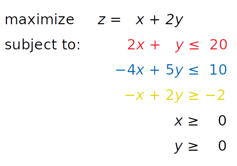
You need to find X and Ÿ The inequality of red, blue and yellow, as well as inequality x ≥ 0 and ⅶ ≥ 0, are satisfactory. At the same time, your solution must correspond to the maximum possible value of z.

The independent variables you need to find (x and y in this case) are called decision variables. The function of the decision variable to maximize or minimize (z in this case) is called objective function, cost function, or just objective. The inequality you need to satisfy is called inequality constraint. You can also use equations in constraints called equality constraints.

This is how you visualize the problem:

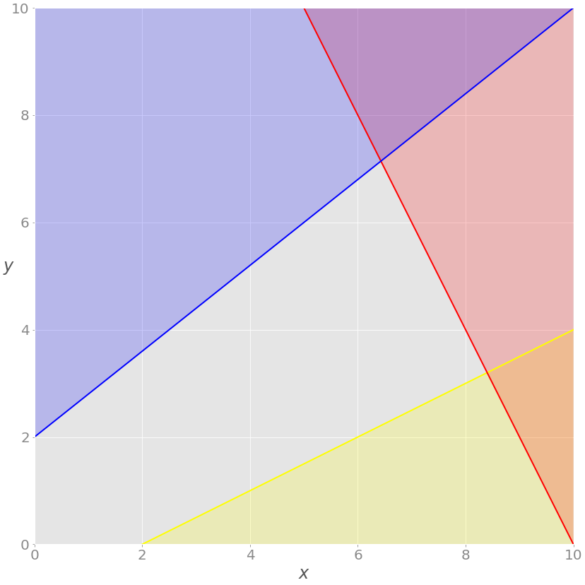
The red line represents the function 2 X+ Ý = 20, and the red area above it shows that the red inequality is not satisfied. Similarly, the blue line is a function − 4 x + 5 y = 10, and the blue area is prohibited because it violates the blue inequality. The yellow line is − x + 2, y = − 2, and the yellow area below it is where the Yellow inequality is invalid.

If you ignore the red, blue, and yellow areas, only the gray areas are retained. Each point in the gray area satisfies all constraints and is a potential solution to the problem. This region is called feasible region, and its point is feasible solution. In this case, there are countless feasible solutions.

You want to maximize z. The feasible solution corresponding to the maximum z is the optimal solution. If you try to minimize the objective function, the best solution will correspond to its feasible minimum.

Notice that z is linear. You can think of it as a plane in three-dimensional space. This is why the optimal solution must be at the vertex or corner of the feasible region. In this case, the best solution is the point where the red and blue lines intersect, as you'll see later.

Sometimes, the entire edge of the feasible region, or even the entire region, can correspond to the same z value. In this case, you have many best solutions.

You are now ready to extend the problem with the additional equality constraints shown in green:

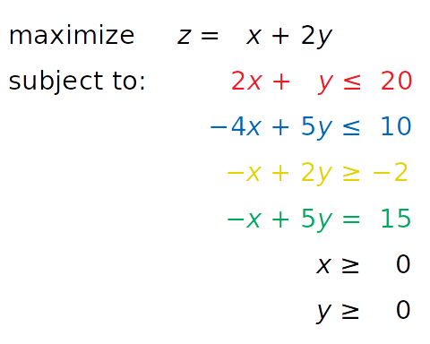
Equation − x + 5, y = 15, written in green, is new. This is an equality constraint. You can visualize the previous image by adding a corresponding green line:

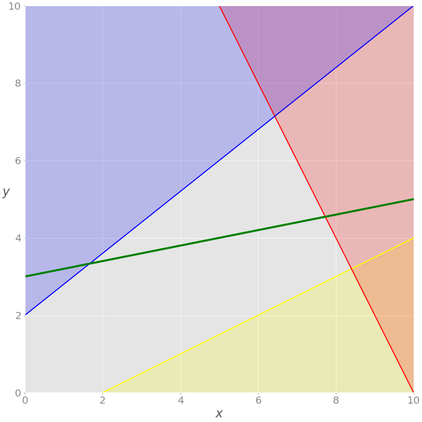
The current solution must satisfy the green equation, so the feasible area is no longer the whole gray area. It is the part where the green line crosses the gray area from the intersection with the blue line to the intersection with the red line. The latter point is the solution.

If all values inserted into x must be integers, then a mixed integer linear programming problem will be obtained, and the set of feasible solutions will change:

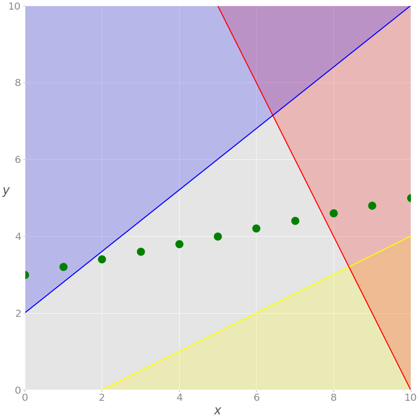
You no longer have a green line, only points along which the x value is an integer. The feasible solution is the green dot on the gray background, and the optimal dissociation red line is the closest.

These three examples illustrate feasible linear programming problems because they have bounded feasible regions and finite solutions.

Infeasible linear programming problem

If there is no solution, the linear programming problem is infeasible. This usually happens when no solution can satisfy all constraints at the same time.

For example, consider what happens if you add a constraint x + y ≤− 1. Then at least one decision variable (x or y) must be negative. This conflicts with the given constraints x ≥ 0 and Y ≥ 0. Such a system has no feasible solution, so it is called infeasible.

Another example is to add a second equality constraint parallel to the green line. These two lines have nothing in common, so there will be no solution that meets these two constraints.

Unbounded linear programming problem

A linear programming problem is unbounded. If its feasible region is unbounded, the solution will not be finite. This means that at least one of your variables is unconstrained and can reach positive infinity or negative infinity, making the goal infinite.

For example, suppose you take the initial question above and remove the red and yellow constraints. Removing constraints from a problem is called a relaxation problem. In this case, x and y are not bounded on the positive side. You can increase them to positive infinity, resulting in infinite z values.

Resource allocation problem

In the previous section, you studied an abstract linear programming problem that is independent of any real application. In this section, you will find more specific and practical optimization problems related to manufacturing resource allocation.

Suppose a factory produces four different products, the daily output of the first product is x ₁, the output of the second product is x 2, and so on. The objective is to determine the profit maximization daily output of each product, bearing in mind the following conditions:

1. The profits per unit product of the first, second, third and fourth products are $20, $12, $40 and $25 respectively.
2. Due to manpower constraints, the total number of units produced per day cannot exceed 50.
3. For the first product per unit, three units of raw material A are consumed. Each unit of second product requires two units of raw material A and one unit of raw material B. Each unit of the third product requires one unit A and two units B. Finally, each unit of the fourth product requires three B units
4. Due to the limitation of transportation and storage, the factory can consume up to 100 units of raw material A and 90 units of B per day.

The mathematical model can be defined as follows:

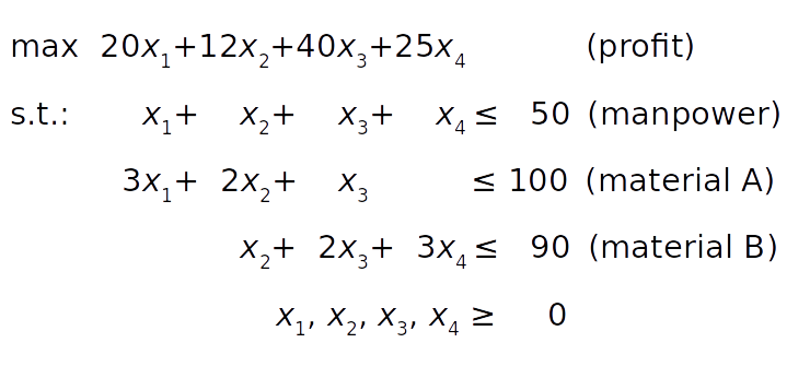
The objective function (profit) is defined in condition 1. The manpower constraint follows condition 2. The constraints on raw materials A and B can be obtained from conditions 3 and 4 by summing the raw material requirements of each product.

Finally, the product quantity cannot be negative, so all decision variables must be greater than or equal to zero.

Unlike the previous example, you cannot easily visualize it because it has four decision variables. However, the principle is the same regardless of the dimension of the problem.

Python implementation of linear programming

In this tutorial, you will use two Python packages to solve the above linear programming problem:

1. SciPy is a generic package for scientific computing using Python.
2. PuLP is a Python linear programming API for defining problems and calling external solvers.

SciPy is easy to set up. After installation, you will have everything you need to get started. Its sub package is SciPy Optimize can be used for linear and nonlinear optimization.

PuLP allows you to select a solver and express the problem in a more natural way. The default solver used by PuLP is COIN-OR Branch and Cut Solver (CBC). It is connected to the COIN-OR linear programming solver (CLP) for linear relaxation and the COIN-OR cut generator Library (CGL) for cut generation.

Another great open source solver is the GNU linear programming Toolkit (GLPK). Some well-known and very powerful commercial and proprietary solutions are Gurobi, CPLEX and XPRESS.

In addition to providing flexibility in defining problems and the ability to run various solvers, PuLP is not as complex to use as alternatives such as Pyomo or CVXOPT, which requires more time and effort to master.

Installing SciPy and PuLP

To learn this tutorial, you need to install SciPy and PuLP. The following example uses SciPy 1.4 Version 1 and PuLP version 2.1.

You can install both using pip:

You may need to run pulptest or sudo pulptest to enable the default solver for PuLP, especially if you are using Linux or Mac:

Alternatively, you can download, install, and use GLPK. It is free and open source for Windows, MacOS, and Linux. Later in this tutorial, you will see how to use GLPK (except CBC) with PuLP.

On Windows, you can download files and run setup files.

On MacOS, you can use Homebrew:

On Debian and Ubuntu, use apt to install glpk and glpk utils:

In Fedora, using dnf has GLPK utils:

You may also find conda useful for installing GLPK:

After installation, you can view the version of GLPK:

For more information, see the GLPK tutorial on installing with Windows executables and Linux packages.

Using SciPy

In this section, you will learn how to use SciPy optimization and rooting library for linear programming.

To use SciPy to define and solve optimization problems, you need to import SciPy optimize. linprog():

Now that you have imported linprog(), you can start optimizing.

Example 1

Let's first solve the above linear programming problem:

linprog() only solves the minimization (not maximization) problem, and does not allow inequality constraints greater than or equal to the sign (≥). To solve these problems, you need to modify your problems before starting optimization:

• Instead of maximizing z = x + 2 y, you can minimize its negative value (− z = − x − 2 y).
• Instead of the greater than or equal sign, you can multiply the Yellow inequality by - 1 and get the opposite number less than or equal to the sign (≤).

After introducing these changes, you will get a new system:

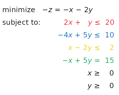
The system is equivalent to the original system and will have the same solution. The only reason to apply these changes is to overcome the limitations of SciPy related to problem representation.

The next step is to define the input values:

You can put the values in the above system into the appropriate list, tuple or NumPy array:

• obj - saves the coefficients of the objective function.
• lhs_ineq # saves the left coefficient of the inequality (red, blue, and yellow) constraint.
• rhs_ineq # saves the right coefficient of the inequality (red, blue, and yellow) constraint.
• lhs_eq ， saves the left coefficient from the equality (green) constraint.
• rhs_eq # saves the right coefficient from the equality (green) constraint.

Note: please pay attention to the order of rows and columns!

The order of rows on the left and right sides of the constraint must be the same. Each row represents a constraint.

The order of the coefficients from the objective function and the left side of the constraint must match. Each column corresponds to a decision variable.

The next step is to define the bounds of each variable in the same order as the coefficients. In this case, they are all between zero and positive infinity:

This statement is redundant because linprog() takes these boundaries (zero to positive infinity) by default.

Note: instead of float("inf"), you can use math inf，numpy.inf or SciPy inf.

Finally, it's time to optimize and solve the problems you are interested in. You can do this linprog():

Parameter c is the coefficient from the objective function. A_ub and b_ub is related to the coefficients on the left and right of inequality constraints, respectively. Similarly, A_eq and b_eq refers to equality constraints. You can use bounds to provide the lower and upper limits of decision variables.

You can use this parameter method to define the linear programming method to be used. There are three options:

1. Method = "interior point" select the interior point method. This option is set by default.
2. method="revised simplex" select the modified two-phase simplex method.
3. method="simplex" select the traditional two-phase simplex method.

linprog() returns a data structure with the following properties:

• . con is the equality constrained residual.
• . fun is the optimal objective function value (if found).
• . message is the status of the solution.
• . nit # is the number of iterations required to complete the calculation.
• . Slack is the value of the slack variable, or the difference between the values on the left and right sides of the constraint.
• . Status is an integer between 0 and 4, which indicates the status of the solution, such as the time when 0 found the best solution.
• . success is a Boolean value indicating whether the best solution has been found.
• . x ， is a NumPy array that holds the optimal value of the decision variable.

You can access these values separately:

This is how you get optimized results. You can also display them graphically:

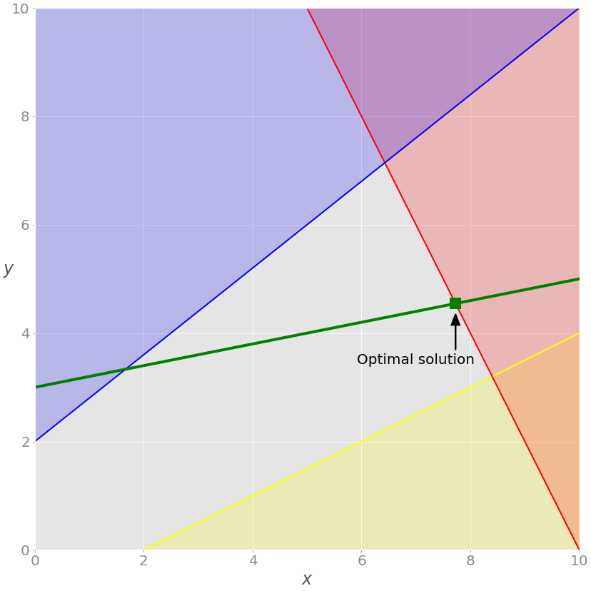
As mentioned earlier, the optimal solution of the linear programming problem is located at the vertex of the feasible region. In this case, the feasible area is only the green line between the blue line and the red line. The optimal solution is a green square representing the intersection of the green line and the red line.

To exclude the equality (green) constraint, simply delete the parameter A_eq and b_eq from the linprog() call:

The solution is different from the previous case. You can see on the chart:

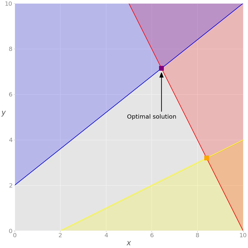
In this example, the optimal solution is the purple vertex of the feasible (gray) region where the red and blue constraints intersect. Other vertices, such as yellow vertices, have higher objective function values.

Example 2

You can use SciPy to solve the resource allocation problem described in the previous section:

As in the previous example, you need to extract the necessary vectors and matrices from the above problem and pass them to as parameters linprog() and get the result:

The result tells you that the maximum profit is 1900 and corresponds to x ₁ = 5 and x ₃ = 45. There is no profit in producing the second and fourth products under given conditions. Here you can draw several interesting conclusions:

1. The third product brings the largest unit profit, so the factory will produce the most.
2. The first slack is 0, which means that the values on the left and right sides of the manpower (first) constraint are the same. The factory produces 50 units per day, which is its full capacity.
3. The second relaxation is 40 because the factory consumes 60 units of raw material A (15 units for the first product and 45100 units for the third product).
4. The third margin is 0, which means that the factory consumes all 90 units of raw material B. All this is for the third product. This is why the factory can not produce the second or fourth product at all, nor can it produce a third product with more than 45 units. Lack of raw materials B

opt.statusis0 and opt Success true indicates that the optimization problem is solved successfully and the optimal feasible solution is obtained.

SciPy's linear programming function is mainly used for smaller problems. For larger and more complex problems, you may find other libraries more suitable for the following reasons:

• SciPy cannot run various external solvers.
• SciPy cannot use integer decision variables.
• SciPy does not provide classes or functions that facilitate model building. You must define arrays and matrices, which can be a tedious and error prone task for large problems.
• SciPy does not allow you to define the maximization problem directly. You must convert them into minimization problems.
• SciPy does not allow you to define constraints directly using the greater than or equal symbol. You must use less than or equal to instead.

Fortunately, the Python ecosystem provides several alternative solutions for linear programming that are useful for larger problems. One of them is PuLP, and you will see its practical application in the next section.

Using PuLP

PuLP has a more convenient linear programming API than SciPy. You don't have to modify your problem mathematically or use vectors and matrices. Everything is cleaner and less error prone.

As usual, you first import what you need:

Now that you have imported PuLP, you can solve your problem.

Example 1

You will now use PuLP to solve this system:

The first step is to initialize an instance LpProblem to represent your model:

You can use this sense parameter to choose whether to minimize (LpMinimize or 1, which is the default) or maximize (LpMaximize or - 1). This choice will affect the result of your problem.

Once you have a model, you can define a decision variable as an instance of the LpVariable class:

You need to provide a lower bound, lowBound=0, because the default value is negative infinity. The parameter upBound defines an upper bound, but you can omit it here because it defaults to positive infinity.

The optional parameter cat defines the category of the decision variable. If you are using Continuous variables, you can use the default value "Continuous".

You can use variables x and y to create additional PuLP objects that represent linear expressions and constraints:

When you multiply a decision variable by a scalar or construct a linear combination of multiple decision variables, you get a pump Lpaffineexpression represents an instance of a linear expression.

Note: you can increase or decrease variables or expressions, and you can multiply their constants, because pulp classes implement some Python special methods, that is, analog-to-digital types__ add__ ()，__ sub__ () and__ mul__ (). These methods are used for behaviors like custom operators +, - and *.

Similarly, you can combine linear expressions, variables, and scalars with the operators = =, < =, or > = to get a representation of the linear constraints of the model LpConstraint instance.

Note: it is also possible to construct constraints with rich comparison methods__ eq__ ()，.__ le__ () and__ ge__ () defines the operator's behavior = =, < = and > =.

With this in mind, the next step is to create constraints and objective functions and assign them to your model. You do not need to create lists or matrices. Just write Python expressions and attach them to the model using the + = operator:

In the code above, you defined a tuple containing the constraint and its name. LpProblem allows you to add constraints to the model by specifying constraints as tuples. The first element is an LpConstraint instance. The second element is the readable name of the constraint.

Setting the objective function is very similar:

Alternatively, you can use shorter symbols:

Now you have added the objective function and defined the model.

Note: you can use the operator to attach a constraint or target to the model, + = because its class LpProblem implements a special method__ iadd__ (), which is used to specify the behavior + =.

For larger problems, lpSum() is usually more convenient to use with lists or other sequences than the repeat + operator. For example, you can add an objective function to a model using the following statement:

It produces the same result as the previous statement.

You can now see the complete definition of this model:

The string representation of the model contains all relevant data: variables, constraints, targets, and their names.

Note: string representation is built by defining special methods__ repr__ (). More details about__ repr__ (), please check the python OOP string conversion:__ repr__vs__str__ .

Finally, you are ready to solve the problem. You can call solve() your model object to do this. If you want to use the default Solver (CBC), you do not need to pass any parameters:

. solve() calls the underlying solver, modifies the model object, and returns the integer state of the solution, 1 if the optimal solution is found. For the remaining status codes, see LpStatus [].

You can get the optimization result as the attribute model. The function value () and the corresponding method value() returns the actual value of the property:

model.objective holds the objective function model The value of constraints, including the value of relaxation variables, and the optimal value of objects x and y with decision variables. model.variables() returns a list of decision variables:

As you can see, this list contains the exact object LpVariable created using the constructor.

The results are roughly the same as what you get with SciPy.

Note: pay attention to this method solve() -- it changes the state of the object, x and y!

You can see which solver is used by calling solver:

The output informs you that the solver is CBC. You did not specify a solver, so PuLP called the default solver.

If you want to run a different solver, you can specify it as a parameter solve(). For example, if you want to use GLPK and already have it installed, you can use solver=GLPK(msg=False) on the last line. Remember, you also need to import it:

Now that you have imported GLPK, you can use it inside solve():

This msg parameter is used to display information from the solver. msg=False disables the display of this message. If you want to include information, simply omit MSG or set msg=True.

Your model is defined and solved, so you can check the results in the same way as in the previous case:

The results obtained using GLPK are almost the same as those obtained using SciPy and CBC.

Let's see which solver is used this time:

As you defined above with the highlighted statement, model Solve (solver = GLPK (MSG = false)), the solver is GLPK.

You can also use PuLP to solve mixed integer linear programming problems. To define an integer or binary variable, simply pass cat="Integer" or cat="Binary" to LpVariable. Everything else remains the same:

In this example, you have an integer variable and get a different result than before:

Nowx is an integer, as specified in the model. (technically, it holds a floating-point value with zero after the decimal point.) this fact changes the whole solution. Let's show this on the chart:

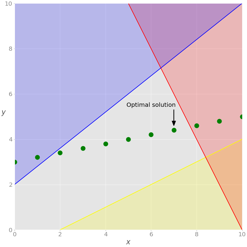
As you can see, the best solution is the rightmost green dot on a gray background. This is the maximum value of both feasible solutions x and y, giving its maximum objective function value.

GLPK can also solve such problems.

Example 2

Now you can use PuLP to solve the above resource allocation problem:

The method of defining and solving the problem is the same as the previous example:

In this case, you use the dictionary x to store all the decision variables. This method is convenient because the dictionary can store the name or index of the decision variable as a key and the corresponding LpVariable object as a value. LpVariable instances of lists or tuples can be useful.

The above code produces the following results:

As you can see, this solution is consistent with the solution obtained using SciPy. The most profitable solution is to produce the first product of 5.0 and the third product of 45.0 every day.

Let's make this problem more complex and interesting. Suppose that due to machine problems, the factory cannot produce the first and third products at the same time. What is the most profitable solution in this case?

Now you have another logical constraint: if x ₁ is a positive number, X ₃ must be zero and vice versa. This is where binary decision variables are very useful. You will use two binary decision variables y ₁ and Y ₃, which will indicate whether the first or third product is generated:

Except for the highlighted lines, the code is very similar to the previous example. Here are the differences:

• Line 5 defines the binary decision variable y[1] and saves y[3] in the dictionary.
• Line 12 defines an arbitrarily large number M. 100 in this case, the value is large enough because you cannot exceed 100 units per day.
• Line 13 says that if y[1] is zero, x[1] must be zero, otherwise it can be any non negative number.
• Line 14 says that if y[3] is zero, x[3] must be zero, otherwise it can be any non negative number.
• Line 15 says either y [1] or [3] is zero (or both), so either x[1]or x[3] must be zero.

This is the solution:

Facts have proved that the best way is to exclude the first product and produce only the third product.

Linear programming solver

Just as there are many resources to help you learn linear programming and mixed integer linear programming, there are many solvers with Python wrappers available. This is a partial list:

• GLPK
• LP Solve
• CLP
• CBC
• CVXOPT
• SciPy
• SCIP with PySCIPOpt
• Gurobi Optimizer
• CPLEX
• XPRESS
• MOSEK

Some of these libraries, such as Gurobi, include their own Python wrappers. Others use external wrappers. For example, you can see that you can use PuLP to access CBC and GLPK.

conclusion

You now know what linear programming is and how to use Python to solve linear programming problems. You also learned that the python linear programming library is just a wrapper for the native solver. When the solver completes its work, the wrapper returns solution state, decision variable value, relaxation variable, objective function, etc.

 

Click focus to learn about Huawei cloud's new technologies for the first time~