catalogue
2. Advantages and disadvantages
2, Decision tree - pick watermelon
1. Create an. ipynb file with jupyter
3, The SK learn library implements the algorithm code of ID3, CART and C4.5 respectively
1, Decision tree
1. Meaning of decision tree:
Decision Tree (Decision Tree) is a decision analysis method that calculates the probability that the expected value of net present value is greater than or equal to zero by forming a Decision Tree on the basis of knowing the occurrence probability of various situations, evaluates the project risk and judges its feasibility. It is a graphical method of intuitively using probability analysis. Because this decision branch is drawn in a graph, it is very similar to the branch of a tree, so it is called Decision Tree In machine learning, the Decision Tree is a prediction model, which represents a mapping relationship between object attributes and object values. Entropy = the disorder degree of the system, using algorithms ID3, C4.5 and C5.0. The spanning tree algorithm uses entropy. This measure is based on the concept of entropy in informatics theory
2. Advantages and disadvantages
advantage:
The decision tree is easy to understand and realize. People do not need users to know a lot of background knowledge in the learning process. At the same time, it can directly reflect the characteristics of data. As long as it is explained, it has the ability to understand the meaning expressed by the decision tree.
For the decision tree, the preparation of data is often simple or unnecessary, and it can deal with data and conventional attributes at the same time, and can make feasible and effective results for large data sources in a relatively short time.
It is easy to evaluate the model through static test and measure the reliability of the model; if an observed model is given, it is easy to deduce the corresponding logical expression according to the generated decision tree.
Disadvantages:
(1) Fields of continuity are difficult to predict.
(2) For data with time sequence, a lot of preprocessing work is required.
(3) When there are too many categories, errors may increase faster.
(4) When the general algorithm classifies, it only classifies according to one field
2, Decision tree - pick watermelon
1. Create an. ipynb file with jupyter
Note: xlrd module and graphviz are used in the process
Wins + R - > CMD enter the following command to download
pip install xlrd
pip install graphviz
2. Code part
#Import module
import pandas as pd
import numpy as np
from collections import Counter
from math import log2
#Data acquisition and processing
def getData(filePath):
data = pd.read_excel(filePath)
return data
def dataDeal(data):
dataList = np.array(data).tolist()
dataSet = [element[1:] for element in dataList]
return dataSet
#Get property name
def getLabels(data):
labels = list(data.columns)[1:-1]
return labels
#Get category tag
def targetClass(dataSet):
classification = set([element[-1] for element in dataSet])
return classification
#Mark the branch node as the leaf node, and select the class with the largest number of samples as the class mark
def majorityRule(dataSet):
mostKind = Counter([element[-1] for element in dataSet]).most_common(1)
majorityKind = mostKind[0][0]
return majorityKind
#Calculating information entropy
def infoEntropy(dataSet):
classColumnCnt = Counter([element[-1] for element in dataSet])
Ent = 0
for symbol in classColumnCnt:
p_k = classColumnCnt[symbol]/len(dataSet)
Ent = Ent-p_k*log2(p_k)
return Ent
#Sub dataset construction
def makeAttributeData(dataSet,value,iColumn):
attributeData = []
for element in dataSet:
if element[iColumn]==value:
row = element[:iColumn]
row.extend(element[iColumn+1:])
attributeData.append(row)
return attributeData
#Calculate information gain
def infoGain(dataSet,iColumn):
Ent = infoEntropy(dataSet)
tempGain = 0.0
attribute = set([element[iColumn] for element in dataSet])
for value in attribute:
attributeData = makeAttributeData(dataSet,value,iColumn)
tempGain = tempGain+len(attributeData)/len(dataSet)*infoEntropy(attributeData)
Gain = Ent-tempGain
return Gain
#Select optimal attribute
def selectOptimalAttribute(dataSet,labels):
bestGain = 0
sequence = 0
for iColumn in range(0,len(labels)):#Ignore the last category column
Gain = infoGain(dataSet,iColumn)
if Gain>bestGain:
bestGain = Gain
sequence = iColumn
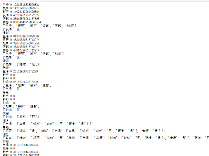
print(labels[iColumn],Gain)
return sequence
#Establish decision tree
def createTree(dataSet,labels):
classification = targetClass(dataSet) #Get category type (collection de duplication)
if len(classification) == 1:
return list(classification)[0]
if len(labels) == 1:
return majorityRule(dataSet)#Return categories with more sample types
sequence = selectOptimalAttribute(dataSet,labels)
print(labels)
optimalAttribute = labels[sequence]
del(labels[sequence])
myTree = {optimalAttribute:{}}
attribute = set([element[sequence] for element in dataSet])
for value in attribute:
print(myTree)
print(value)
subLabels = labels[:]
myTree[optimalAttribute][value] = \
createTree(makeAttributeData(dataSet,value,sequence),subLabels)
return myTree
def main():
filePath = 'xg.xls'
data = getData(filePath)
dataSet = dataDeal(data)
labels = getLabels(data)
myTree = createTree(dataSet,labels)
return myTree
if __name__ == '__main__':
myTree = main()
Output results:
3, The SK learn library implements the algorithm code of ID3, CART and C4.5 respectively
1.ID3 algorithm
Import library and export
Code part:
#Import related libraries
import pandas as pd
import graphviz
from sklearn.model_selection import train_test_split
from sklearn import tree
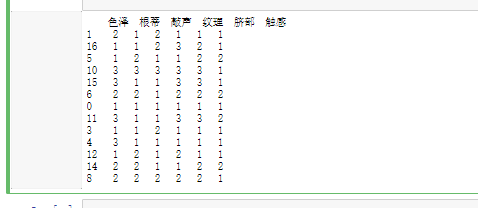
f = open('watermalon.csv','r')
data = pd.read_csv(f)
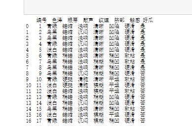
x = data[["color and lustre","Root","stroke ","texture","Umbilicus","Tactile sensation"]].copy()
y = data['Good melon'].copy()
print(data)
Result diagram:
Convert data (since the data contains Chinese characters, further processing of the data is required)
#Numeric eigenvalues
x = x.copy()
for i in ["color and lustre","Root","stroke ","texture","Umbilicus","Tactile sensation"]:
for j in range(len(x)):
if(x[i][j] == "dark green" or x[i][j] == "Curl up" or data[i][j] == "Turbid sound" \
or x[i][j] == "clear" or x[i][j] == "sunken" or x[i][j] == "Hard slip"):
x[i][j] = 1
elif(x[i][j] == "Black" or x[i][j] == "Slightly curled" or data[i][j] == "Dull" \
or x[i][j] == "Slightly paste" or x[i][j] == "Slightly concave" or x[i][j] == "Soft sticky"):
x[i][j] = 2
else:
x[i][j] = 3
y = y.copy()
for i in range(len(y)):
if(y[i] == "yes"):
y[i] = int(1)
else:
y[i] = int(-1)
#You need to convert the data x and y into a good format and the data frame dataframe, otherwise the format will report an error
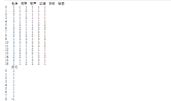
x = pd.DataFrame(x).astype(int)
y = pd.DataFrame(y).astype(int)
print(x)
print(y)Result diagram:
Modeling and training
x_train, x_test, y_train, y_test = train_test_split(x,y,test_size=0.2)
print(x_train)
Result diagram
Training results
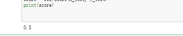
clf = tree.DecisionTreeClassifier(criterion="entropy")                    #instantiation
clf = clf.fit(x_train, y_train)
score = clf.score(x_test, y_test)
print(score)
Result diagram:
2.C4.5 algorithm
In order to solve the disadvantages of ID3 algorithm, C4.5 algorithm is produced. C4.5 algorithm is similar to ID3 algorithm, but the difference is that C4.5 algorithm adopts information gain ratio as the standard when selecting features.
ID3 algorithm has four main shortcomings:
① Continuous features cannot be processed
② Using the information gain as the standard is easy to favor the characteristics with more values
③ Missing value processing
④ Over fitting problem
For the fourth problem, C4.5 introduces the regularization coefficient for preliminary pruning.
Information gain ratio
The information gain criterion has a preference for attributes with a large number of values. In order to reduce the possible adverse effects of this preference, C4.5 algorithm uses the information gain rate to select the optimal partition attribute. Gain rate formula

among , K values. If A is used to divide sample set D, K branch nodes will be generated, in which the k-th node contains all attributes in D, and the value on A is  A sample of is recorded as
  . Generally, the more possible values of attribute A (i.e. the greater K), the greater the value of IV(A).
The information gain rate criterion has a preference for attributes with a small number of values. Therefore, C4.5 algorithm does not directly select the candidate partition attribute with the largest information gain rate, but first find the attribute with higher information gain than the average level from the candidate partition attributes, and then select the attribute with the highest information gain rate.
Processing of continuous features
When the attribute type is discrete, there is no need to discretize the data;
When the attribute type is continuous, the data needs to be discretized. The specific ideas are as follows:
Specific ideas:
- The continuous characteristic a of M samples has m values, which are arranged A1, A2,... Am from small to large , Take the average of two adjacent sample values as the division point, there are m-1 in total, and the ith division point Ti is expressed as:
 .
. - Calculate the information gain rate when taking these m-1 points as binary segmentation points respectively. Select the point with the largest information gain rate as the best segmentation point of the continuous feature. For example, the point with the largest information gain rate is at , Then less than
 The value of is category 1, greater than The value of is category 2, so the discretization of continuous features is achieved.
Handling of missing values
ID3 algorithm cannot handle missing values, while C4.5 algorithm can handle missing values (commonly used probability weight method). There are three main cases, as follows:
- How to calculate the information gain rate on features with missing values?
According to the missing ratio, convert the information gain (the proportion of samples without missing values multiplied by the information gain of the subset of samples without missing values) and the information gain rate
2. If the division attribute is selected, how to divide the sample if the value of the sample on this attribute is missing?
The samples are divided into different nodes at the same time with different probabilities. The probability is obtained according to the proportion of other non missing attributes
3. When classifying new samples, how to judge the category if there are missing values in the characteristics of test samples?
Take all branches, calculate the probability of each category, and assign the category with the greatest probability to the sample
3.CART algorithm
1. Understanding of cart algorithm
Classification And Regression Tree, i.e. Classification And Regression Tree algorithm, referred to as CART algorithm, is an implementation of decision tree. Generally, there are three main implementations of decision tree, namely ID3 algorithm, CART algorithm and C4.5 algorithm. CART algorithm is a binary recursive segmentation technology, which divides the current sample into two sub samples, so that each non leaf node has two branches. Therefore, the decision tree generated by CART algorithm is a binary tree with simple structure. Because CART algorithm is a binary tree, it can only be "yes" or "no" in each step of decision-making. Even if a feature has multiple values, it also divides the data into two parts. The CART algorithm is mainly divided into two steps
(1) Recursive partition of samples for tree building process
(2) Pruning with validation data
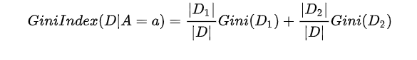
2. Gini coefficient
The purity of data set D can be measured by Gini value

Among them,  Is classification
  Probability of occurrence, n is the number of classifications. Gini(D) reflects the probability that two samples are randomly selected from data set D and their category labels are inconsistent. Therefore, the smaller Gini(D), the higher the purity of data set D.
For sample D, the number is | D | and sample D is divided into two parts according to whether feature a takes a possible value a D1 and D2 . Therefore, CART classification tree algorithm establishes a binary tree, not a multi binary tree. 
Under the condition of attribute A, the Gini coefficient of sample D is defined as
Processing of continuous and discrete features
For the continuous value processing of CART classification tree, its idea is the same as C4.5, which discretizes the continuous features. The only difference lies in the different measurement methods when selecting partition points. C4.5 uses information gain, and CART classification tree uses Gini coefficient.
The specific idea is as follows. For example, there are m continuous features a of M samples, which are arranged from small to large as a1,a2,...,ama1,a2,...,am, then the CART algorithm takes the median of the values of two adjacent samples and obtains m-1 partition points, in which the ith partition point Ti represents Ti as: Ti=ai+ai+12Ti=ai+ai+12. For these m-1 points, the Gini coefficients when the point is used as the binary classification point are calculated respectively. The point with the smallest Gini coefficient is selected as the binary discrete classification point of the continuous feature. For example, if the lowest Gini coefficient is atat, the value less than atat is category 1 and the value greater than atat is category 2. In this way, we can discretize the continuous features. It should be noted that, unlike discrete attributes, if the current node is a continuous attribute, the attribute can also participate in the generation and selection process of child nodes.
The idea of dealing with the discrete value of CART classification tree is the non-stop binary discrete feature. CART classification tree will consider dividing a into {A1} and {A2,A3}{A1} and {A2,A3},{A2} and {A1,A3}{A2} and {A1,A3},{A3} and {A1,A2}{A3} and {A1,A2} to find the combination with the smallest Gini coefficient, such as {A2} and {A1,A3} and {A1,A3}, and then establish binary tree nodes. One node is the sample corresponding to A2 and the other node is the node corresponding to {A1,A3}. At the same time, since the values of feature a are not completely separated this time, we still have the opportunity to continue to select feature a at the child node to divide A1 and A3. This is different from ID3 or C4.5. In a subtree of ID3 or C4.5, discrete features will only participate in the establishment of nodes once.
4, Summary
Through this experiment, I learned about the use of ID3, C4.5 and cart, as well as their advantages and disadvantages.
reference:
ID3 and C4.5 of decision tree generation
Decision tree algorithm - C4.5 algorithm - Zhihu (zhihu.com)