Week Learning Notes (2021.8.2-2021.8.8)
8.2
Mainly around datawhale Used Car Transaction Price Forecast Contest Learning Content
Official FAQ Suddenly found that the official FAQs (Frequently Asked Questions FAQs) are excellent. Unlike other FAQs in other contests, they focus on learning and can learn a lot.
1. Macro Average-Micro Average
For multi-classification problems
Macro Average, Fine Precision to Number
There are two formulas for calculating the value of macro F1, keeping an eye on the indicators given in the competition
2. Typeora shortcuts
ctrl+shift+m insertion formula
ctrl+i tilt
ctrl+u underline
3. CTR & CVR
(1)CTR
CTR (Click-Through-Rate) is a term commonly used in Internet advertising. It refers to the click-through rate of an online advertisement (picture/text/keyword/ranking/video, etc.), that is, the actual number of clicks (strictly speaking, the number of pages that reach the target) divided by the amount of Show content displayed in the advertisement.
c
t
r
=
spot
hit
second
number
spot
hit
amount
ctr=\frac{hits}{hits}
ctr = clicks
(2)CVR
CVR (Conversion Rate): Conversion rate. CPA is a measure of the effectiveness of CPA advertising. In short, it is the rate at which users click on an advertisement to become an active, registered or even paying user.
c
v
r
=
spot
hit
amount
turn
turn
amount
cvr=\frac{hits}{conversions}
cvr = conversion hits
4. Evaluation Index
from sklearn.metrics import
accuracy_score precision_score recall_score f1_score roc_auc_score
(y_true,y_pred)
#Note: roc_auc_score(y_true,y_pred) can only calculate AUC values, not draw ROC curves
(1) Classification tasks
-
TP TN FN FP
-
acc precision recall (both molecule are TP)
acc is susceptible to sample size and sample balance
precision denominator is TP+FP for all samples with positive predictions
The recall denominator is all true canonicals, TP+FN - we need to get back samples that were not predicted correctly but were positive in themselves, called recalls
-
f1
Accuracy and recall rates go from one another, so f1 values need to be reconciled
Product of double and sum
-
PR Curve ROC Curve AUC
P, R in PR curve is Precision, Recall
Advantages of ROC: ROC curves can remain unchanged when positive and negative sample distributions are inconsistent
-
logloss
-(ylog§+(1-y)log(1-p))
Where y denotes the true label of the sample and p denotes the probability that the model predicts a positive sample
(2) Regression task
from sklearn.metrics import
mean_squared_error mean_absolute_error r2_score
-
Mean absolute error mean absolute error
-
MSE (mean square error) mean square error
-
RMSE (root mean square error) root mean square error (root of MSE directly)
np.sqrt(mean_squared_error(y_true,y_pred))
-
MAPE (mean absolute percentage error) average absolute percentage error
def mape(y_true,y_pred): return np.mean(np.abs((y_pred-y_true)/y_true)) -
R-side
5. Outliers from numerical variable analysis - data.describe()
Don't just think that there may be outliers for object types, but also for float s and int s in info(), value_counts may be too inconvenient, so you can use data.describe()
Two benefits: a quick grasp of the approximate extent of the data; Strange numbers like 99999 or -1 may also be outliers and need to be replaced with np.nan
8.3
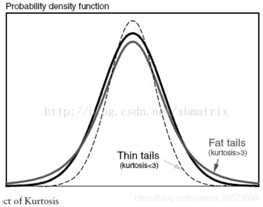
1. Skewness and kurtosis of regression problems
Why check skewness and kurtosis?
Skewness and kurtosis combined with standard errors can be used to test whether the data follows a normal distribution, whether it is left or right, or to make it normal based on the ratio between them.
. skew() and. Both kurt() can act directly on the Seres type
Normal distribution (skewness = 0), Right skewed distribution (positive skewness distribution, skewness > 0), Left skewed distribution (negative skewness distribution, skewness < 0)
Normal distribution (kurtosis = 0), thick tail (kurtosis > 0), thin tail (kurtosis < 0)
Low-peak datasets are scattered and have more extreme values. Peak data sets are more concentrated, with less data on both sides
2. Gauss distribution (normal distribution)
Why should the target variable be as Gaussian as possible?
Because there are many algorithms that assume that the data is normally distributed, for example, one of the assumptions of the least quadratic method in linear regression is that the data is normally distributed.
3. Category characteristics are severely skewed
Usually such features do not play a role in model prediction and are recommended to be deleted
Don't have to have value_for every feature Counts()
The quickest and most intuitive way to do this is to draw a histogram of each feature
4. Common Visualizations
(1) Bar chart
x,y,data,hue,order parameters with Violin and box plots
sns.barplot(x="color",y="age",data=data)
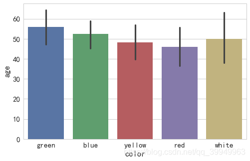
Interpretation of Images
After sorting the values in the "color" column, Seaborn calculates the corresponding values according to the **estimator parameter ** (default is average) method, and the calculated values are displayed as bars (error bars on bars indicate errors between values of each type relative to those shown on bars).
Explanation of Error Lines
Error lines are derived from statistics and represent the range of data errors (or uncertainties) to present data in a more accurate way. Error lines can be expressed as standard deviation (SD), standard error (SE), and confidence intervals, and either representation can be used and explained accordingly. When the error lines are longer, the data is either more discrete or has fewer data samples.
The estimator controls what values the entire column of data is drawn with, the default mean, and the median np.median
ci confidence interval (0-100), if set to "sd", use standard deviation (default 95% confidence interval) - related to error lines
(2) Count chart
The countplot parameter and barplot are almost the same, but count() cannot enter both x and y, and countplot has no error lines
(3) Histogram + Kernel Density Estimation Map
Form subboxes along the data range, drawing bars to show the data distribution of the number of observations falling into each subbox
Adjust whether histograms and kernel density estimates are displayed by hist and kde parameters (default hist and kde are True)
fit controls the fitted parameter distribution graph to visually evaluate its relationship with the observed data
sns.distplot(x,color="g",hist=True,kde=True,fit=norm)
(4) Map of kernel density estimation
Visually see the distribution of the sample itself
shade defaults to False, meaning no shadow
vertical defaults to False, meaning drawn on the x-axis
sns.kdeplot(x,color="g")
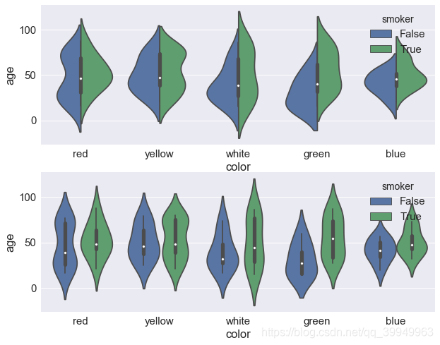
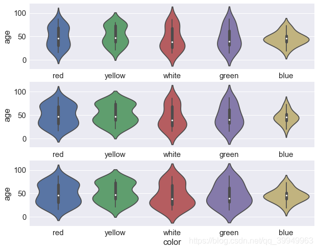
(5) Violin drawings
X, y, hue, data, order, palette (palette), orient parameters and box plot usage are the same
Split sets it to true and draws a split violinplot to compare the two quantities split by hue
fig,axes=plt.subplots(2,1)
ax=sns.violinplot(x="color",y="age",data=data,hue="smoker",split=True,ax=axes[0])
ax=sns.violinplot(x="color",y="age",data=data,hue="smoker",ax=axes[1])
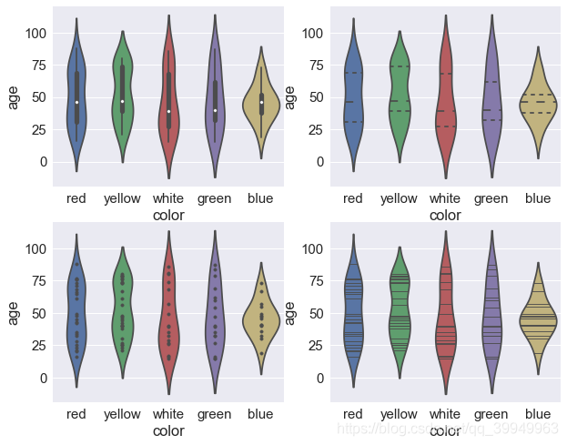
inner controls the representation of violinplot internal data points in four ways:'box','quartile','point','stick'
fig,axes=plt.subplots(2,2)
sns.violinplot(x="color",y="age",data=data,inner="box",ax=axes[0,0])  #Box plot inside violin (top left)
sns.violinplot(x="color",y="age",data=data,inner="quartile",ax=axes[0,1])  #Piano diagram with quartile line (top right)
sns.violinplot(x="color",y="age",data=data,inner="point",ax=axes[1,0])  #Piano Picture with specific data points (bottom left)
sns.violinplot(x="color",y="age",data=data,inner="stick",ax=axes[1,1])  #Piano Picture with Data Bar (bottom right)
scale scales the width of each violin in three ways: area,count,width
fig,axes=plt.subplots(3,1)
sns.violinplot(x="color",y="age",data=data,scale="area",ax=axes[0]) #If it is an area, each violin will have the same area (above)
sns.violinplot(x="color",y="age",data=data,scale="count",ax=axes[1])  #If it is count, the width of the violin will be scaled according to the amount observed in the group (middle)
sns.violinplot(x="color",y="age",data=data,scale="width",ax=axes[2])  #If it is "age", each violin will have the same width (below)
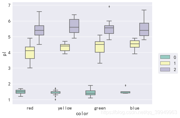
(6) Box plot
Column name (str) or vector data in x,y dataframe
data dataframe or array
Column name of hue dataframe, classified by the values in the column name to form a classified bar chart
y should be considered a target attribute, x is a non-target attribute, and hue is another non-target attribute. That is, two variables nest groupby()
Order controls the order of the bar graph (x-axis)
sns.boxplot(x="color",y="pl",data=data,hue="catagory")
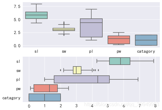
orient'v'|'h' is used to control whether the image is displayed horizontally or vertically (typically when x, y are not passed in and only data is passed in)
fig,axes=plt.subplots(2,1)
sns.boxplot(data=data,orient="v",ax=axes[0])
sns.boxplot(data=data,orient="h",ax=axes[1])
(7) Missing visualization
import missingno as msno
(8) Visualization Report
import pandas_profiling
pfr=pandas_profiling.ProfileReport(Train_data)
pfr.to_file()
(9) Presenting multiple pictures at the same time
fig,axes=plt.subplots(1,3)
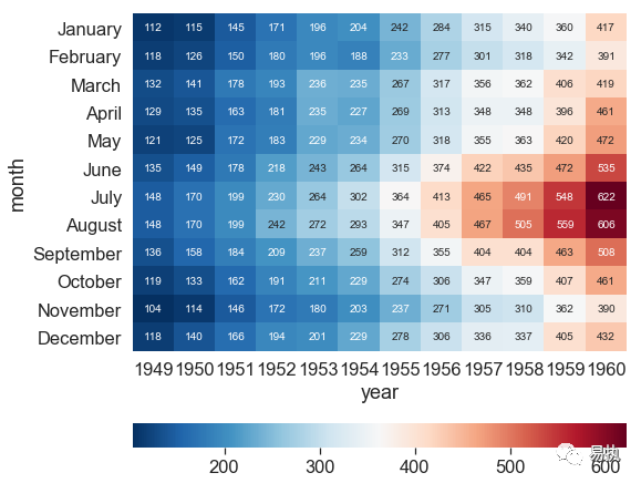
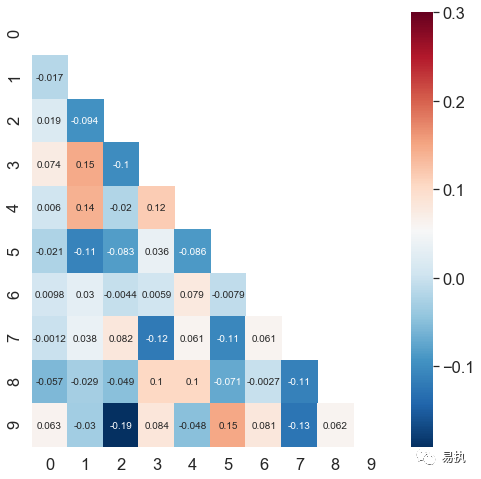
(10) Thermograph
The dividing line of the center color band
Whether annot displays numeric annotations, defaulting to False; And the numeric notes default to scientific counting, which can be confusing if viewed too long. You can format the FMT parameter as an abbreviation for format, fmt="d" integer
linewidths controls the spacing between each small square
square bool type, whether to make each cell square, defaults to False
sns.heatmap()
cbar_kws settings for color bands, default portrait
cbar_kws={"orientation":"horizontal"} #Display color band horizontally
mask passes into a Boolean matrix, and if True is present in the matrix, the corresponding data of the thermogram will be blocked.
# correlation coefficent correlation coefficient
corr=np.corrcoef(data) #Generating correlation coefficient matrices for datasets
mask=np.zeros_like(corr) # Generate a matrix of all zeros in the shape of corr
mask[np.triu_indices_from(mask)] = True #Set the mask diagonal and above to True
#np.triu_indices_from() gets the serial number
mask=mask #Incoming parameters
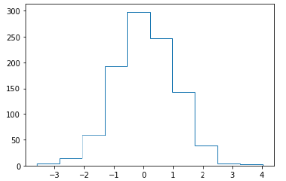
(11) Histogram
bins controls the number of intervals divided in the histogram, simply passing in the number
Color controls the fill color of columns
The DENSITE parameter defaults to False, which means that the number of values per interval is used to plot the column. When the value is True, the height of the column is the frequency of each interval.
The orientation parameter defaults to vertical, meaning that columns are drawn upright. Draw horizontal columns when horizontal
histtype specifies the type of histogram to draw, defaulting to bar, "step" represents the line of the border
plt.hist(x,bins,color,density,orientation,histtype)
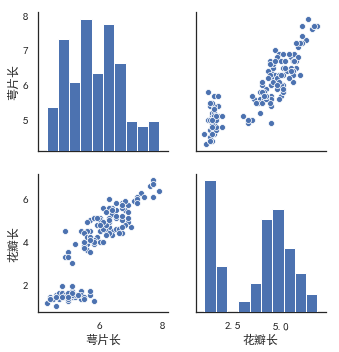
(12) the relationship between two pairgrids ()
kind controls the type of diagonal graph, "scatter" "reg"
Scatter scatter plot
"reg" fits a straight line to a scatterplot of non-diagonal lines
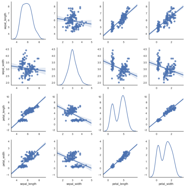
diag_kind controls the type of graph on the diagonal line, "hist""kde" (diagonal)
hue is generally a target attribute
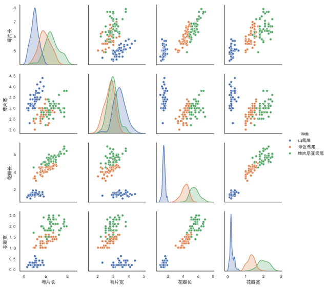
When vars relates one or more variables, a list parameter is passed in
sns.pairplot(data,kind,diag_kind,hue,vars)
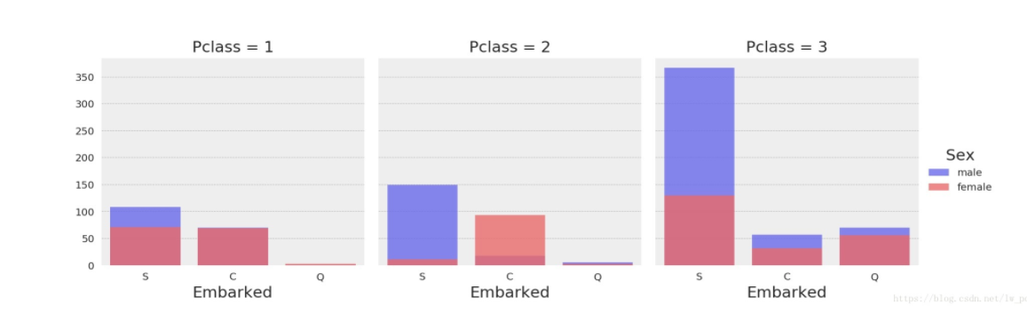
(13) the relationship between multiple variables facetgrid()
Use SNS first. FacetGrid adjusts its parameters and then draws the image directly using map functionality
Note: The map() function passes in two parameters, one is the function name and the other is an iterative object, such as a list, tuple
col passes in a string of non-target attribute column names that can be drawn in string categories, one of which belongs, and the horizontal coordinates are useful
g=sns.FacetGrid(data,col="",hue="")
g.map(plt.scatter,"Transverse coordinates","Ordinate coordinates",alpha=)
#Parameters can be added to the second line statement

sns.set(font_scale=2) #Adjust Font in Text
# Number comparison of men and women at different ports of landing at different social levels
grid = sns.FacetGrid(data_all, col='Pclass', hue='Sex', palette='seismic', size=4)
# 'Embarked'is data_ Field in all (is a DataFrame)
grid.map(sns.countplot, 'Embarked', alpha=.8)
# A legend appears on the right side of the graph
grid.add_legend()
5. Correlation coefficient matrix
data.corr() #The correlation coefficient between any two variables
If you want to see the relationship between a non-target variable and a target variable, you can directly index the column of the target variable in the correlation coefficient matrix and sort it
correlation=data.corr()
correlation["price"].sort_values(ascending=False) #Sort dependencies from large to small (linear relationships only)
#Ascending stands for ascending order
8.4
1. str.cat()
Column a name. Str.cat (column B name)
Both columns are of string type before they can be merged
Connectors can be set in cat() to facilitate subsequent separation of sep=''
You can convert a numeric variable to a character type at this point
df['price']=df['price'].astype('str')
df['price']=df['price'].map(lambda x:str(x))
2. Feature Screening
Benefits:
1. Reduce dimension, make the model more generalized and reduce overfitting
2. Remove irrelevant features and reduce learning difficulty
In most cases, the embedded method is chosen for feature filtering, and the filter can also see the correlation coefficient initially
- filter: Select the features of the data before training the learner. The common methods are Relief/Variance Selection/Correlation Coefficient/Chi-square Test/Mutual Information.
Remove features of low variance
Sort the correlation coefficients, calculate the correlation coefficients between each feature and the target variable, set a threshold, and select the features whose correlation coefficients are greater than this threshold.
Use hypothesis tests to get the correlation between features and output values, such as chi-square test, T-test, F-test
Using mutual information to analyze correlation from the perspective of information entropy
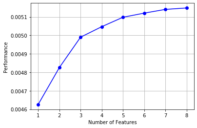
- Wapper: Direct evaluation of the performance of the **learner that will eventually be used** as a subset of features, common methods being LVM (Las Vegas Wrapper)
Continuously select a subset of features from the initial feature set, train the learner, and evaluate the subset based on the performance of the learner until the best subset is selected
Advantages: From the performance of the final learner, wrapped is better than filtered
Disadvantages: multiple training sessions are required and computational overhead is greater than filtering
Most likely, the Las Vegas Wrapper uses a random strategy for subset searches. Using random strategies, each feature subset evaluation requires a training learner, which is expensive to compute and has drawbacks.
Consequently, greedy algorithms are commonly used, such as forward search (which incrementally adds features on the optimal subset until they no longer improve model performance), backward search, and two-way search (a combination of forward and backward).
!pip install mlxtend

from mlxtend.feature_selection import SequentialFeatureSelector as SFS
from sklearn.linear_model import LinearRegression
sfs = SFS(LinearRegression(),
           k_features=10,
           forward=True,
           floating=False,
           scoring = 'r2',
           cv = 0)
x = data.drop(['price'], axis=1)
x = x.fillna(0)
y = data['price']
sfs.fit(x, y)
sfs.k_feature_names_

#output
('powerPS_ten',
 'city',
 'brand_price_std',
 'vehicleType_andere',
 'model_145',
 'model_601',
 'fuelType_andere',
 'notRepairedDamage_ja')
# If you draw it, you can see the marginal benefit
from mlxtend.plotting import plot_sequential_feature_selection as plot_sfs
import matplotlib.pyplot as plt
fig1 = plot_sfs(sfs.get_metric_dict(), kind='std_dev')
plt.grid()
plt.show()
-
embedding: Combining filter and package, the trainer automatically makes feature selection during training. The common ones are lasso regression, ridge regression and decision tree.
In the filter and package feature selection methods, there is a clear difference between the feature selection and the learning process. However, embedding embeds the feature selection algorithm itself as a component in the learning algorithm, that is, feature selection is automatically performed during the training process of the learner.
Using regularization, the feature coefficient becomes zero to achieve feature selection
Only an algorithm that derives the feature coefficients or the importance of features can be used as a base learner for embedded selection
3. Truncated outliers
The upper limit of box plot Q3+1.5IQR; Lower limit Q1-1.5IQR
"""Here's a wrapper of exception handling code that you can call anywhere"""
def outliers_proc(data, col_name, scale=3):
    """
        Used to truncate outliers, by default box_plot(scale=3)Cleaning, not dealing with outliers, but with extremes
        param:
            data:  Receive pandas data format
            col_name: pandas Column Name
            scale: scale
    """
    data_col = data[col_name]
    Q1 = data_col.quantile(0.25) # 0.25 Quantile
    Q3 = data_col.quantile(0.75)  # 0,75 Quantiles
    IQR = Q3 - Q1

    data_col[data_col < Q1 - (scale * IQR)] = Q1 - (scale * IQR) #Processing Lower Limit Data
    data_col[data_col > Q3 + (scale * IQR)] = Q3 + (scale * IQR) #Processing upper bound data

    return data[col_name]

num_data['power'] = outliers_proc(num_data, 'power')
Explain why scale is usually 3

4. pd.to_datetime()
Converts the object type to the datetime type (time type), so the format parameter matches the original string
There are formats in the data that have time errors, so we need errors='coerce'purpose: encounter settings that cannot be converted to nan
Subtract two variables of type datetime to get the number of days, and for type Series, dt.days transformation
data['used_time'] = (pd.to_datetime(data['creatDate'], format='%Y%m%d', errors='coerce') -
                            pd.to_datetime(data['regDate'], format='%Y%m%d', errors='coerce')).dt.days
5.round()
Round (numeric value, decimal places preserved)
6. Benefits of data bucketing
(1) Faster operation of product within sparse vectors after discretization
(2) The discretized features are more robust to outliers because an outlier is divided into barrels.
(3) LR is a generalized linear model with limited expressive power. After discretization, each variable has a separate weight, which is equivalent to the introduction of non-linearity, which can improve the expressive power of the model and increase the fit
(4) After discretization, features can be crossed to enhance the expression ability. M*N variables are programmed by M+N variables, and non-linear shape is introduced to further improve the expression ability.
(5) The model is more stable when the features are discrete, such as the age range of users, which will not change as the users get older than one year.
7. Convert a dictionary to a dataframe
Dictionary contains a nested dictionary, that is, dictionary elements are dictionaries, outermost keys are column names, and inner keys are row names.
8. data.columns
Although not referenced, if the index needs to become a list tolist(), you can always know the data column name
9. First step in drawing
f , ax = plt.subplots(figsize = (7, 7))
10. Ways to reduce memory for large datasets
#An ancestor function that can be used directly
def reduce_mem_usage(df):
    """ iterate through all the columns of a dataframe and modify the data type
        to reduce memory usage.
    """
    start_mem = df.memory_usage().sum()  #Calculate the original dataframe data memory
    print('Memory usage of dataframe is {:.2f} MB'.format(start_mem))

    for col in df.columns:
        col_type = df[col].dtype  #Series column has the same data type

        if col_type != object:  #If not a string
            c_min = df[col].min()  #minimum value
            c_max = df[col].max()  #Maximum
            if str(col_type)[:3] == 'int':  #Complete type is int64, top 3
                #np.iinfo() shows machine limits of integer type
                if c_min > np.iinfo(np.int8).min and c_max < np.iinfo(np.int8).max:
                #If it can be in the range of int8, shrink to np.int8
                    df[col] = df[col].astype(np.int8)
                elif c_min > np.iinfo(np.int16).min and c_max < np.iinfo(np.int16).max:
                    df[col] = df[col].astype(np.int16)
                elif c_min > np.iinfo(np.int32).min and c_max < np.iinfo(np.int32).max:
                    df[col] = df[col].astype(np.int32)
                elif c_min > np.iinfo(np.int64).min and c_max < np.iinfo(np.int64).max:
                    df[col] = df[col].astype(np.int64)
            else:
                if c_min > np.finfo(np.float16).min and c_max < np.finfo(np.float16).max:
                    df[col] = df[col].astype(np.float16)
                elif c_min > np.finfo(np.float32).min and c_max < np.finfo(np.float32).max:
                    df[col] = df[col].astype(np.float32)
                else:
                    df[col] = df[col].astype(np.float64)
        else:
            df[col] = df[col].astype('category') #Change from object to category type

    end_mem = df.memory_usage().sum()  #Calculate memory size after conversion
    print('Memory usage after optimization is: {:.2f} MB'.format(end_mem))
    print('Decreased by {:.1f}%'.format(100 * (start_mem - end_mem) / start_mem)) #Percentage of memory change
    return df


sample_feature = reduce_mem_usage(pd.read_csv('data_for_tree.csv'))
11. dtype() & astype() &type()
type() returns ** data structure type **
Note that the word "structure" is used to store data
list,dict,tuple
dtype() returns ** data type **
dtype() cannot be called because list s, dict s may contain different data types
np.array requires all elements to be of the same data type, so dtype() can be called
int64 float64 object
astype() changes np. Data type of all data elements in array
You can use dtype() to use astype()
Note: Series'underlying data is built by ndarray, the difference is the Series serial number
12. Normal distribution in data preprocessing
13. np.iinfo()
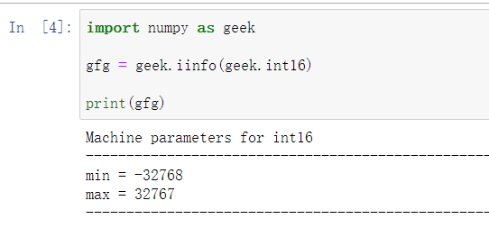
Output is fantastic, but you can use gfg. Min() & gfg. Max() gets the minimum and maximum values
14. category() & object()
Change from object() to category() to speed up
15. reset_index()
Replace the original sequence, reorder, start at 0
Two important parameters
drop parameter, default is False, delete original index column set to True
Inplace parameter, inplace=True is required to modify the original data
16. LinearRegession() parameter
LinearRegression(fit_intercept=True, normalize=False, copy_X=True, n_jobs=None)
fit_intercept:bool type, whether there is intercept, if not, a straight line crosses the origin;
Normalize: whether to normalize the data;
copy_X: Default to True, when True, X will be copied, otherwise X will be overwritten;
n_jobs: The default value is 1. Number of cores used in calculation
#View the intercept and coef of the training linear regression model
'intercept:'+ str(model.intercept_)

#Reverse from large to small means reverse, so true means descending
sorted(dict(zip(continuous_feature_names, model.coef_)).items(), key=lambda x:x[1], reverse=True)
Interpret:
zip() packages the corresponding elements in the object into a tuple and returns the list
dict() makes tuple pairs in lists dictionary-like
. items() returns a list whose elements are tuples
8.5
1. Dictionary d.values () & d.keys () & d.items ()
There will always be dict_in front of it Values, dict_keys, dict_ The items prefix, the list in parentheses, uses the list() function to get a pure list
2. sorted() & sort()
(1)sort()
The reverse parameter controls ascending and descending order, has no return value, and operates directly on the list
a=[1,4,88,5,2]
a.sort() #Default ascending sort
a.sort(reverse=False) #Equivalent to
(2)sorted()
There is also a reverse parameter with a return value
b=sorted(a)
Note: Use of the parameter key in the function
When the elements in the list are no longer single, if the list contains tuples or dictionaries
[Tuples included in list]
key=lambda x:x[0] #Sort by first
[Dictionary included in list]
Sort by a key value in the dictionary
key=lambda x:x[key value]
3. Learning Curve-Verification Curve
The learning curve refers to the comparison of the score of the training set and the verification set when the parameter values are determined to see whether the model state is under- or over-fit
Complexity curves (validation set curves) show the comparison of training set and test set scores for a parameter at different values
Model complexity is small, then under-fitting will occur
If the model is complex, it will be overfitted
4. np.nan_to_num()
nan not a number
Replace the nan element in array x with 0, and the inf element with a finite number
5. reshape(m,-1)
This function can only be used on matrices or arrays, -1 means automatic calculation, that is, the number of all elements in a matrix/array divided by m
Number of rows and columns, respectively
6. Return value of cross-validation function
from sklearn.model_selection import cross_val_score
from sklearn.metrics import mean_absolute_error,make_scorer
scores=cross_val_score(model,X=train_x,y=train_y,verbose=1,cv=5,
                       scoring=make_scorer(mean_absolute_error(y_true,y_pred)))
This scores has five values because cv=5
7. np.linspace()
Generate equal difference column, return array type
train_size=np.linspace(start,stop,num,endpoint,retstep,dtype,axis)
9. Regularize L1 L2
[What is each L1 L2 regularization]

Normally a coefficient is added before the regularization term
[Regularization effect]

[Sparse Model]
Sparse models remove a large number of redundant variables, leaving only the explanatory variables most relevant to the response variables.
Simplifies the model while retaining the most important information in the dataset, effectively solving many problems in high-dimensional dataset modeling
Sparse models are more explanatory, making it easier to visualize data, reduce computation, and transfer storage
Sparse models are related to feature selection because if the coefficients are or are small, even if they are removed, they have no effect on the model.
9. split()
Returns a delimited list
10. MLP (Multilayer Sensor)
11. Master the parameters of three GBDT models
xgboost
catboost
lightgbm
12. Model Tuning
(1) Greedy parametric adjustment (coordinate descent)
Step: Establish a list for each parameter, with list elements as optional parameters; Create a dictionary for each parameter, storing parameter values and current cross-validation averages
#Example, call LGBMRegressor()
best_obj = dict()
for obj in objective:
    model = LGBMRegressor(objective=obj)
    score = np.mean(cross_val_score(model, X=train_X, y=train_y_ln, verbose=0, cv = 5, scoring=make_scorer(mean_absolute_error)))
    best_obj[obj] = score

best_leaves = dict()
for leaves in num_leaves:
    model = LGBMRegressor(objective=min(best_obj.items(), key=lambda x:x[1])[0], num_leaves=leaves)
    score = np.mean(cross_val_score(model, X=train_X, y=train_y_ln, verbose=0, cv = 5, scoring=make_scorer(mean_absolute_error)))  #For each parameter is a 50 percent average
    best_leaves[leaves] = score

best_depth = dict() #A Dictionary of parameters of this type, with each key-value pair and one score for each key
for depth in max_depth:
    model = LGBMRegressor(objective=min(best_obj.items(), key=lambda x:x[1])[0],
                          num_leaves=min(best_leaves.items(), key=lambda x:x[1])[0],
                          max_depth=depth)
    score = np.mean(cross_val_score(model, X=train_X, y=train_y_ln, verbose=0, cv = 5, scoring=make_scorer(mean_absolute_error)))
    best_depth[depth] = score
(2) Grid search
The essence of grid search is to assemble, combine the possible values of each variable, and have fewer or more parameters, but more parameters will take a lot of time, so you can select a large range before filtering.
clf is the abbreviation of classifier
parameters={'objective':objective,'num_leaves':num_leaves,'max_depth':max_depth}
model=LGBMRegressor()
clf=GridSearchCV(model,parameters,cv=5) #Choose the best model
clf=clf.fit(train_X,train_y)
[Common Properties]
clf.best_params_ Parameter combinations describing the best results achieved
clf.best_score_ Provides the best score observed during optimization
(3) Bayesian tuning
[To be improved]
Advantages: Using a Gaussian process, considering previous information, continuously updating a priori, while grid search does not take into account previous parameter information
Bayesian tuning iteration is less and slower
(4) RandomizedSearchCV random search
8.6
1. Data Contest - Model
(1) Artificially specifying model parameters
Types that can be put directly into a model after data processing --> Set model parameters, and return values are marked as models
model=LinearRegression(normalize=True)
->Train labeled data (training set) with a model and record the return value again
model=model.fit(train_x,train_y)
Prediction using this model (artificially specified is a superparameter, and one parameter is learned in fit)
(2) Automatically adjusting parameters to determine the best combination of superparameters
8.7
1. LOOCV & K-foldCV
cv cross validation cross validation
Reference DataWhale
trade-off for bias and variance means the balance of deviation and variance
In fact, LOOCV is a special K-fold Cross Validation (K=N). The last K selection is a trade-off** of ** Bias and Variance. The larger the K, the more data is put into the training set each time, the smaller the Bias of the model. However, the larger the K, the greater the correlation before each selected training set. (Consider the most extreme example, when k = N, that is, in LOOCV, the training data is almost the same each time). This large correlation results in a larger Variance for the final test error. Typically, choose 5 or 10 for the K value.
2. GridSearchCV Supplement
The essence is violent search, which works in small datasets but not in large ones. Large amounts of data can use a fast tuning method, coordinate descent, which is essentially a greedy algorithm, to tune the parameters that currently have the greatest impact on the model, to reach the optimal solution, and then to tune the next parameter that has a greater impact on the model until all the parameters have been adjusted.
Advantages: Time and effort saving
Disadvantages: Move to local optimum instead of global optimum
8.8
_ Parameter combinations describing the best results achieved
clf.best_score_ Provides the best score observed during optimization
(3) Bayesian tuning
[To be improved]
Advantages: Using a Gaussian process, considering previous information, continuously updating a priori, while grid search does not take into account previous parameter information
Bayesian tuning iteration is less and slower
(4) RandomizedSearchCV random search
8.6
1. Data Contest - Model
(1) Artificially specifying model parameters
Types that can be put directly into a model after data processing --> Set model parameters, and return values are marked as models
model=LinearRegression(normalize=True)
->Train labeled data (training set) with a model and record the return value again
model=model.fit(train_x,train_y)
Prediction using this model (artificially specified is a superparameter, and one parameter is learned in fit)
(2) Automatically adjusting parameters to determine the best combination of superparameters
8.7
1. LOOCV & K-foldCV
cv cross validation cross validation
Reference DataWhale
trade-off for bias and variance means the balance of deviation and variance
In fact, LOOCV is a special K-fold Cross Validation (K=N). The last K selection is a trade-off** of ** Bias and Variance. The larger the K, the more data is put into the training set each time, the smaller the Bias of the model. However, the larger the K, the greater the correlation before each selected training set. (Consider the most extreme example, when k = N, that is, in LOOCV, the training data is almost the same each time). This large correlation results in a larger Variance for the final test error. Typically, choose 5 or 10 for the K value.
2. GridSearchCV Supplement
The essence is violent search, which works in small datasets but not in large ones. Large amounts of data can use a fast tuning method, coordinate descent, which is essentially a greedy algorithm, to tune the parameters that currently have the greatest impact on the model, to reach the optimal solution, and then to tune the next parameter that has a greater impact on the model until all the parameters have been adjusted.
Advantages: Time and effort saving
Disadvantages: Move to local optimum instead of global optimum
8.8
Not learning