Reference link: https://blog.csdn.net/u013733326/article/details/79702148
Prepare package
We need to prepare some software packages:
- numpy: it is a basic software package for scientific computing in Python.
- sklearn: a simple and efficient tool for data mining and data analysis.
- matplotlib: is a library for drawing charts in Python.
- testCases: some test examples are provided to evaluate the correctness of the function. See the downloaded materials or check its code at the bottom.
- planar_utils: provides various useful functions used in this task. See the downloaded materials or check its code at the bottom.
# Prepare package
import numpy as np
import matplotlib.pyplot as plt
from testCases import *
import sklearn
import sklearn.datasets
import sklearn.linear_model
from planar_utils import plot_decision_boundary, sigmoid, load_planar_dataset, load_extra_datasets

%matplotlib inline #If you use Jupiter notebook, please uncomment it.

np.random.seed(1) #Set a fixed random seed to ensure that our results are consistent in the next steps.
Output:
UsageError: unrecognized arguments: #If you use Jupiter notebook, please uncomment it.
Loading and viewing datasets
#View dataset
X, Y = load_planar_dataset()

#Visual dataset
plt.scatter(X[0, :], X[1, :], c=Y, s=40, cmap=plt.cm.Spectral) #Scatter plot

# If there is a problem with the previous sentence, please use the following statement:
# plt.scatter(X[0, :], X[1, :], c=np.squeeze(Y), s=40, cmap=plt.cm.Spectral) #Scatter plot
Output:
<matplotlib.collections.PathCollection at 0x1ab3d993a08>
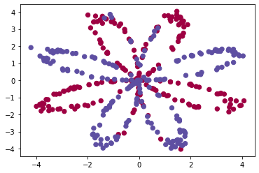
The data looks like a flower pattern of red (y = 0) and some blue (y = 1) data points. Our goal is to build a model to adapt to these data. Now, we have the following things:
- 10: A numpy matrix containing the values of these data points
- Y: A numpy vector corresponds to the label of X [0 | 1] (red: 0, blue: 1)
#View data types
shape_X = X.shape
shape_Y = Y.shape
m = Y.shape[1]  # Number in training set

print ("X The dimension of is: " + str(shape_X))
print ("Y The dimension of is: " + str(shape_Y))
print ("The data in the dataset includes:" + str(m) + " individual")
Output:
X The dimension of is: (2, 400)
Y The dimension of is: (1, 400)
There are 400 data in the dataset
See the classification effect of simple Logistic regression
Before building a complete neural network, let's see how logistic regression performs on this problem. We can use the built-in function of sklearn to do this, and run the following code to train the logistic regression classifier on the data set.
# Construct Logistic regression model and train the model at the same time
clf = sklearn.linear_model.LogisticRegressionCV()
clf.fit(X.T,Y.T)
Output:
LogisticRegressionCV()
# Draw classification effect
plot_decision_boundary(lambda x: clf.predict(x), X, Y) #Draw decision boundaries
plt.title("Logistic Regression") #Icon question
LR_predictions  = clf.predict(X.T) #Prediction results
print ("Accuracy of logistic regression: %d " % float((np.dot(Y, LR_predictions) +
                                np.dot(1 - Y,1 - LR_predictions)) / float(Y.size) * 100) +
       "% " + "(Percentage of correctly marked data points)") # Divide the sum of positive and negative predictions by the total to get the percentage
Output:
Accuracy of logistic regression: 47 % (Percentage of correctly marked data points)
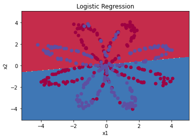
The reason for the accuracy of only 47% is that the data set is not linearly separable, so the performance of logistic regression is poor. Now we officially start to build neural network.
Build neural network
The general method of constructing neural network is:
- Define the neural network structure (number of input units, number of hidden units, etc.).
- Initialize the parameters of the model
- Cycle:
- Implement forward communication
- Calculate loss
- Backward propagation
- Update parameters (gradient descent)
We want them to merge into one NN_ In the model () function, when we build nn_model() and learn the correct parameters, we can predict the new data.
Define neural network structure
Before construction, we need to define the structure of neural network:
- n_x: Enter the number of layers
- n_h: Number of hidden layers (set to 4 here)
- n_y: Number of output layers
def layer_sizes(X , Y):
    """
    Parameters:
     X - Input dataset,Dimension is (quantity entered, training)/Number of tests)
     Y - Label, dimension is (output quantity, training)/Number of tests)

    return:
     n_x - Enter the number of layers
     n_h - Number of hidden layers
     n_y - Number of output layers
    """
    n_x = X.shape[0] #Input layer
    n_h = 4 #, hidden layer, hard coded as 4
    n_y = Y.shape[0] #Output layer

    return (n_x,n_h,n_y)
# Test neural network structure
print("=========================test layer_sizes=========================")
X_asses , Y_asses = layer_sizes_test_case() #Random initialization X_asses and Y_asses
(n_x,n_h,n_y) =  layer_sizes(X_asses,Y_asses)
print("The number of nodes in the input layer is: n_x = " + str(n_x))
print("The number of nodes in the hidden layer is: n_h = " + str(n_h))
print("The number of nodes in the output layer is: n_y = " + str(n_y))
Output:
=========================test layer_sizes=========================
The number of nodes in the input layer is: n_x = 5
 The number of nodes in the hidden layer is: n_h = 4
 The number of nodes in the output layer is: n_y = 2
Initialize the parameters of the model
Here, we want to implement the function initialize_parameters(). We should ensure that our parameters are of appropriate size. If necessary, please refer to the neural network diagram above.
We will initialize the weight matrix with random values.
- np.random.randn(a, b)* 0.01 to randomly initialize a matrix with dimension (a, b).
Initializes the bias to zero.
- np.zeros((a, b)) initializes the matrix (a, b) with zero.
def initialize_parameters( n_x , n_h ,n_y):
    """
    Parameters:
        n_x - Enter the number of layer nodes
        n_h - Number of hidden layer nodes
        n_y - Number of output layer nodes

    return:
        parameters - Dictionary with parameters:
            W1 - Weight matrix,Dimension is( n_h,n_x)
            b1 - Bias, dimension( n_h,1)
            W2 - Weight matrix, dimension( n_y,n_h)
            b2 - Bias, dimension( n_y,1)

    """
    np.random.seed(2) #Specify a random seed so that your output is the same as ours.
    # Random initialization weight
    W1 = np.random.randn(n_h,n_x) * 0.01
    b1 = np.zeros(shape=(n_h, 1))
    W2 = np.random.randn(n_y,n_h) * 0.01
    b2 = np.zeros(shape=(n_y, 1))

    #Use assertions to ensure that my data format is correct
    assert(W1.shape == ( n_h , n_x ))
    assert(b1.shape == ( n_h , 1 ))
    assert(W2.shape == ( n_y , n_h ))
    assert(b2.shape == ( n_y , 1 ))

    parameters = {"W1" : W1,
                  "b1" : b1,
                  "W2" : W2,
                  "b2" : b2 }

    return parameters
#Test initialize_parameters
print("=========================test initialize_parameters=========================")
n_x , n_h , n_y = initialize_parameters_test_case() #n_x, n_h, n_y = 2, 4, 1
parameters = initialize_parameters(n_x , n_h , n_y)
print("W1 = " + str(parameters["W1"]))
print("b1 = " + str(parameters["b1"]))
print("W2 = " + str(parameters["W2"]))
print("b2 = " + str(parameters["b2"]))
Output:
=========================test initialize_parameters=========================
W1 = [[-0.00416758 -0.00056267]
 [-0.02136196  0.01640271]
 [-0.01793436 -0.00841747]
 [ 0.00502881 -0.01245288]]
b1 = [[0.]
 [0.]
 [0.]
 [0.]]
W2 = [[-0.01057952 -0.00909008  0.00551454  0.02292208]]
b2 = [[0.]]
loop
Forward propagation
def forward_propagation( X , parameters ):
    """
    Parameters:
         X - Dimension is( n_x,m)Input data for.
         parameters - Initialization function( initialize_parameters)Output of

    return:
         A2 - use sigmoid()The value after the second activation of the function calculation
         cache - Contain“ Z1","A1","Z2"And“ A2"Dictionary type variable for
     """
    # Obtain weight matrix
    W1 = parameters["W1"]
    b1 = parameters["b1"]
    W2 = parameters["W2"]
    b2 = parameters["b2"]
    # Forward propagation calculation A2
    Z1 = np.dot(W1 , X) + b1
    A1 = np.tanh(Z1)
    Z2 = np.dot(W2 , A1) + b2
    A2 = sigmoid(Z2)
    # Use assertions to ensure that my data format is correct
    assert(A2.shape == (1,X.shape[1]))
    # Integration results
    cache = {"Z1": Z1,
             "A1": A1,
             "Z2": Z2,
             "A2": A2}

    return (A2, cache)
#Test forward_propagation
print("=========================test forward_propagation=========================")
X_assess, parameters = forward_propagation_test_case()
A2, cache = forward_propagation(X_assess, parameters)
print(np.mean(cache["Z1"]), np.mean(cache["A1"]), np.mean(cache["Z2"]), np.mean(cache["A2"]))
Output:
=========================test forward_propagation=========================
-0.0004997557777419902 -0.000496963353231779 0.00043818745095914653 0.500109546852431
Calculate loss
# logprobs = np.multiply(np.log(A2),Y)
# cost = - np.sum(logprobs)                # It can be calculated directly without using a loop.
def compute_cost(A2,Y,parameters):
    """
    Calculate the cross entropy cost given in equation (6),

    Parameters:
         A2 - use sigmoid()The value after the second activation of the function calculation
         Y - "True"Label vector,Dimension is (1, quantity)
         parameters - A contains W1,B1,W2 and B2 Variable of dictionary type

    return:
         cost - Cross entropy cost gives equation (13)
    """
    m = Y.shape[1]  #Number of samples
    # Get the masses
    W1 = parameters["W1"]
    W2 = parameters["W2"]

    #Calculate cost
    logprobs = np.multiply(np.log(A2), Y) + np.multiply((1 - Y), np.log(1 - A2))
    cost = - np.sum(logprobs) / m #Average
    cost = float(np.squeeze(cost)) #Convert to float type

    # Determine whether the cross entropy cost is a floating point number
    assert(isinstance(cost,float))

    return cost
#Test compute_cost
print("=========================test compute_cost=========================")
A2 , Y_assess , parameters = compute_cost_test_case()
print("cost = " + str(compute_cost(A2,Y_assess,parameters)))
Output:
=========================test compute_cost=========================
cost = 0.6929198937761266
Backward propagation
def backward_propagation(parameters,cache,X,Y):
    """
    Use the above instructions to build the back propagation function.

    Parameters:
     parameters - A dictionary type variable containing our parameters.
     cache - Contain“ Z1","A1","Z2"And“ A2"A variable of dictionary type.
     X - Input data, dimension is (2, quantity)
     Y - "True"Label, dimension is (1, quantity)

    return:
     grads - contain W and b The derivative of a dictionary type variable.
    """
    # Number of samples obtained
    m = X.shape[1]

    # Obtain weight matrix
    W1 = parameters["W1"]
    W2 = parameters["W2"]

    #Obtain the output of each layer
    A1 = cache["A1"]
    A2 = cache["A2"]

    dZ2= A2 - Y #calculation error
    dW2 = (1 / m) * np.dot(dZ2, A1.T)
    db2 = (1 / m) * np.sum(dZ2, axis=1, keepdims=True)
    dZ1 = np.multiply(np.dot(W2.T, dZ2), 1 - np.power(A1, 2))
    dW1 = (1 / m) * np.dot(dZ1, X.T)
    db1 = (1 / m) * np.sum(dZ1, axis=1, keepdims=True)

    # Get the partial derivative of each layer
    grads = {"dW1": dW1,
             "db1": db1,
             "dW2": dW2,
             "db2": db2 }

    return grads
#Test backward_propagation
print("=========================test backward_propagation=========================")
parameters, cache, X_assess, Y_assess = backward_propagation_test_case()

grads = backward_propagation(parameters, cache, X_assess, Y_assess)
print ("dW1 = "+ str(grads["dW1"]))
print ("db1 = "+ str(grads["db1"]))
print ("dW2 = "+ str(grads["dW2"]))
print ("db2 = "+ str(grads["db2"]))
Output:
=========================test backward_propagation=========================
dW1 = [[ 0.01018708 -0.00708701]
 [ 0.00873447 -0.0060768 ]
 [-0.00530847  0.00369379]
 [-0.02206365  0.01535126]]
db1 = [[-0.00069728]
 [-0.00060606]
 [ 0.000364  ]
 [ 0.00151207]]
dW2 = [[ 0.00363613  0.03153604  0.01162914 -0.01318316]]
db2 = [[0.06589489]]
Update parameters
def update_parameters(parameters,grads,learning_rate=1.2):
    """
    Update the parameters using the gradient descent update rule given above

    Parameters:
     parameters - A variable that contains the dictionary type of the parameter.
     grads - A variable of dictionary type containing derivative values.
     learning_rate - Learning rate

    return:
     parameters - A variable that contains the dictionary type of the update parameter.
    """
    # Get weight
    W1,W2 = parameters["W1"],parameters["W2"]
    b1,b2 = parameters["b1"],parameters["b2"]

    # Get all derivatives
    dW1,dW2 = grads["dW1"],grads["dW2"]
    db1,db2 = grads["db1"],grads["db2"]

    # Update weight
    W1 = W1 - learning_rate * dW1
    b1 = b1 - learning_rate * db1
    W2 = W2 - learning_rate * dW2
    b2 = b2 - learning_rate * db2

    parameters = {"W1": W1,
                  "b1": b1,
                  "W2": W2,
                  "b2": b2}

    return parameters
#Test update_parameters
print("=========================test update_parameters=========================")
parameters, grads = update_parameters_test_case()
parameters = update_parameters(parameters, grads)

print("W1 = " + str(parameters["W1"]))
print("b1 = " + str(parameters["b1"]))
print("W2 = " + str(parameters["W2"]))
print("b2 = " + str(parameters["b2"]))
Output:
=========================test update_parameters=========================
W1 = [[-0.00643025  0.01936718]
 [-0.02410458  0.03978052]
 [-0.01653973 -0.02096177]
 [ 0.01046864 -0.05990141]]
b1 = [[-1.02420756e-06]
 [ 1.27373948e-05]
 [ 8.32996807e-07]
 [-3.20136836e-06]]
W2 = [[-0.01041081 -0.04463285  0.01758031  0.04747113]]
b2 = [[0.00010457]]
integration
We now integrate the above into NN_ In model (), the neural network model must use the previous functions in the correct order.
def nn_model(X,Y,n_h,num_iterations,print_cost=False):
    """
    Parameters:
        X - data set,Dimension is (2, number of examples)
        Y - Label, dimension is (1, number of examples)
        n_h - Number of hidden layers
        num_iterations - Number of iterations in gradient descent cycle
        print_cost - If yes True,Then the cost value is printed every 1000 iterations

    return:
        parameters - Model learning parameters that can be used for prediction.
     """

    np.random.seed(3) #Specify random seed
    n_x = layer_sizes(X, Y)[0] #Input layer
    n_y = layer_sizes(X, Y)[2] #Output layer

    #Initialize weight
    parameters = initialize_parameters(n_x,n_h,n_y)
    W1 = parameters["W1"]
    b1 = parameters["b1"]
    W2 = parameters["W2"]
    b2 = parameters["b2"]

    #Gradient descent
    for i in range(num_iterations):
        A2 , cache = forward_propagation(X,parameters) #Forward propagation
        cost = compute_cost(A2,Y,parameters) #Calculate cost function value
        grads = backward_propagation(parameters,cache,X,Y) #Back propagation
        parameters = update_parameters(parameters,grads,learning_rate = 0.5) #Update gradient

        #Determine whether to output
        if print_cost:
            if i%1000 == 0:
                print("The first ",i," Cycle, cost:"+str(cost))
    return parameters
#Test nn_model
print("=========================test nn_model=========================")
X_assess, Y_assess = nn_model_test_case()

parameters = nn_model(X_assess, Y_assess, 4, num_iterations=10000, print_cost=False)
print("W1 = " + str(parameters["W1"]))
print("b1 = " + str(parameters["b1"]))
print("W2 = " + str(parameters["W2"]))
print("b2 = " + str(parameters["b2"]))
Output:
=========================test nn_model=========================
W1 = [[-3.89167767  4.77541602]
 [-6.77960338  1.20272585]
 [-3.88338966  4.78028666]
 [ 6.77958203 -1.20272574]]
b1 = [[ 2.11530892]
 [ 3.41221357]
 [ 2.11585732]
 [-3.41221322]]
W2 = [[-2512.9093032  -2502.70799785 -2512.01655969  2502.65264416]]
b2 = [[-22.29071761]]
forecast
predict() is built to predict using the model, and forward propagation is used to predict the results.
def predict(parameters,X):
    """
    Use the learned parameters for X Each example in predicts a class

    Parameters:
        parameters - A variable that contains the dictionary type of the parameter.
        X - Input data( n_x,m)

    return
        predictions - Vector predicted by our model (red: 0 /Blue: 1)

    """
    # The predicted value can be obtained by forward propagation of the incoming data and weight
    A2 , cache = forward_propagation(X, parameters)
    predictions = np.round(A2) # Take 0.5 as the boundary to predict

    return predictions
#Test predict
print("=========================test predict=========================")

parameters, X_assess = predict_test_case()

predictions = predict(parameters, X_assess)
print("Forecast average = " + str(np.mean(predictions)))
Output:
=========================test predict=========================
Forecast average = 0.6666666666666666
Formal operation
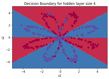
parameters = nn_model(X, Y, n_h = 4, num_iterations=10000, print_cost=True)
#Draw boundary
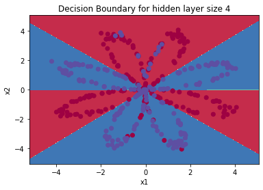
plot_decision_boundary(lambda x: predict(parameters, x.T), X, Y)
plt.title("Decision Boundary for hidden layer size " + str(4))
predictions = predict(parameters, X)
print ('Accuracy: %d' % float((np.dot(Y, predictions.T) + np.dot(1 - Y, 1 - predictions.T)) / float(Y.size) * 100) + '%')
Output:
Cycle 0, cost: 0.6930480201239823
 Cycle 1000, cost: 0.3098018601352803
 Cycle 2000, cost: 0.2924326333792646
 Cycle 3000, cost: 0.2833492852647412
 Cycle 4000, cost: 0.27678077562979253
 Cycle 5000, cost: 0.26347155088593144
 Cycle 6000, cost: 0.24204413129940763
 Cycle 7000, cost: 0.23552486626608762
 Cycle 8000, cost: 0.23140964509854278
 Cycle 9000, cost: 0.22846408048352365
 Accuracy: 90%
Change the number of hidden layer nodes
In the above experiment, we set the hidden layer as four nodes. Now we change the number of nodes in the hidden layer to see whether the number of nodes will affect the results.
plt.figure(figsize=(16, 32))
hidden_layer_sizes = [1, 2, 3, 4, 5, 20, 50] #Number of hidden layers
for i, n_h in enumerate(hidden_layer_sizes):
    plt.subplot(5, 2, i + 1)
    plt.title('Hidden Layer of size %d' % n_h)
    parameters = nn_model(X, Y, n_h, num_iterations=5000)
    plot_decision_boundary(lambda x: predict(parameters, x.T), X, Y)
    predictions = predict(parameters, X)
    accuracy = float((np.dot(Y, predictions.T) + np.dot(1 - Y, 1 - predictions.T)) / float(Y.size) * 100)
    print ("Number of hidden layer nodes: {}  ,Accuracy: {} %".format(n_h, accuracy))
Output:
Number of nodes in hidden layer: 1, accuracy: 67.25 %
Number of nodes in hidden layer: 2, accuracy: 66.5 %
Number of nodes in hidden layer: 3, accuracy: 89.25 %
Number of nodes in hidden layer: 4, accuracy: 90.0 %
Number of nodes in hidden layer: 5, accuracy: 89.75 %
Number of nodes in hidden layer: 20, accuracy: 90.0 %
Number of nodes in hidden layer: 50, accuracy: 89.75 %
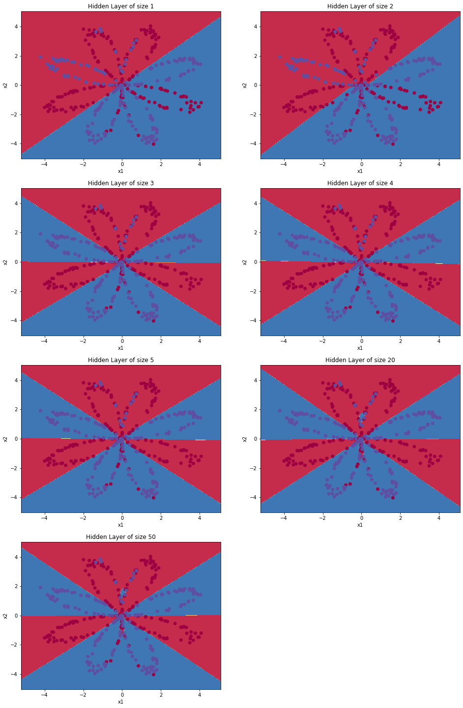
Larger models (with more hidden units) can better adapt to the training set until the final maximum model over fits the data.
The best hidden layer size seems to be n_ H = near 5. In fact, the values here seem to fit the data well and will not cause over fitting.
We will also learn about regularization later, which allows us to use very large models (such as n_h = 50) without too much over fitting.
Change learning_ What happens to the rate value
Change the learning rate of 0.5 to 0.1
def nn_model(X,Y,n_h,num_iterations,print_cost=False):
    """
    Parameters:
        X - data set,Dimension is (2, number of examples)
        Y - Label, dimension is (1, number of examples)
        n_h - Number of hidden layers
        num_iterations - Number of iterations in gradient descent cycle
        print_cost - If yes True,Then the cost value is printed every 1000 iterations

    return:
        parameters - Model learning parameters that can be used for prediction.
     """

    np.random.seed(3) #Specify random seed
    n_x = layer_sizes(X, Y)[0] #Input layer
    n_y = layer_sizes(X, Y)[2] #Output layer

    #Initialize weight
    parameters = initialize_parameters(n_x,n_h,n_y)
    W1 = parameters["W1"]
    b1 = parameters["b1"]
    W2 = parameters["W2"]
    b2 = parameters["b2"]

    #Gradient descent
    for i in range(num_iterations):
        A2 , cache = forward_propagation(X,parameters) #Forward propagation
        cost = compute_cost(A2,Y,parameters) #Calculate cost function value
        grads = backward_propagation(parameters,cache,X,Y) #Back propagation
        parameters = update_parameters(parameters,grads,learning_rate = 0.1) #Update gradient

        #Determine whether to output
        if print_cost:
            if i%1000 == 0:
                print("The first ",i," Cycle, cost:"+str(cost))
    return parameters
parameters = nn_model(X, Y, n_h = 4, num_iterations=10000, print_cost=True)

#Draw boundary
plot_decision_boundary(lambda x: predict(parameters, x.T), X, Y)
plt.title("Decision Boundary for hidden layer size " + str(4))

predictions = predict(parameters, X)
print ('Accuracy: %d' % float((np.dot(Y, predictions.T) + np.dot(1 - Y, 1 - predictions.T)) / float(Y.size) * 100) + '%')
Output:
Cycle 0, cost: 0.6930480201239823
 Cycle 1000, cost: 0.6082072899772629
 Cycle 2000, cost: 0.36073810801711914
 Cycle 3000, cost: 0.3290211712344614
 Cycle 4000, cost: 0.3169254361704178
 Cycle 5000, cost: 0.3097334282605931
 Cycle 6000, cost: 0.3046867806714765
 Cycle 7000, cost: 0.3008037341117686
 Cycle 8000, cost: 0.29763181251528925
 Cycle 9000, cost: 0.2949307617619345
 Accuracy: 89%
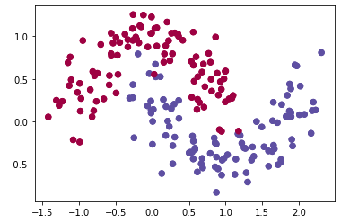
What if we change the dataset?
# data set
noisy_circles, noisy_moons, blobs, gaussian_quantiles, no_structure = load_extra_datasets()

datasets = {"noisy_circles": noisy_circles,
            "noisy_moons": noisy_moons,
            "blobs": blobs,
            "gaussian_quantiles": gaussian_quantiles}

dataset = "noisy_moons"

X, Y = datasets[dataset]
X, Y = X.T, Y.reshape(1, Y.shape[0])

if dataset == "blobs":
    Y = Y % 2

plt.scatter(X[0, :], X[1, :], c=Y, s=40, cmap=plt.cm.Spectral)

#If there is a problem with the previous sentence, please use the following statement:
plt.scatter(X[0, :], X[1, :], c=np.squeeze(Y), s=40, cmap=plt.cm.Spectral)
Output:
<matplotlib.collections.PathCollection at 0x1ab3f620388>
planar_utils.py
import matplotlib.pyplot as plt
import numpy as np
import sklearn
import sklearn.datasets
import sklearn.linear_model

def plot_decision_boundary(model, X, y):
    # Set min and max values and give it some padding
    x_min, x_max = X[0, :].min() - 1, X[0, :].max() + 1
    y_min, y_max = X[1, :].min() - 1, X[1, :].max() + 1
    h = 0.01
    # Generate a grid of points with distance h between them
    xx, yy = np.meshgrid(np.arange(x_min, x_max, h), np.arange(y_min, y_max, h))
    # Predict the function value for the whole grid
    Z = model(np.c_[xx.ravel(), yy.ravel()])
    Z = Z.reshape(xx.shape)
    # Plot the contour and training examples
    plt.contourf(xx, yy, Z, cmap=plt.cm.Spectral)
    plt.ylabel('x2')
    plt.xlabel('x1')
    plt.scatter(X[0, :], X[1, :], c=y, cmap=plt.cm.Spectral)


def sigmoid(x):
    s = 1/(1+np.exp(-x))
    return s

def load_planar_dataset():
    np.random.seed(1)
    m = 400 # number of examples
    N = int(m/2) # number of points per class
    D = 2 # dimensionality
    X = np.zeros((m,D)) # data matrix where each row is a single example
    Y = np.zeros((m,1), dtype='uint8') # labels vector (0 for red, 1 for blue)
    a = 4 # maximum ray of the flower

    for j in range(2):
        ix = range(N*j,N*(j+1))
        t = np.linspace(j*3.12,(j+1)*3.12,N) + np.random.randn(N)*0.2 # theta
        r = a*np.sin(4*t) + np.random.randn(N)*0.2 # radius
        X[ix] = np.c_[r*np.sin(t), r*np.cos(t)]
        Y[ix] = j

    X = X.T
    Y = Y.T

    return X, Y

def load_extra_datasets():
    N = 200
    noisy_circles = sklearn.datasets.make_circles(n_samples=N, factor=.5, noise=.3)
    noisy_moons = sklearn.datasets.make_moons(n_samples=N, noise=.2)
    blobs = sklearn.datasets.make_blobs(n_samples=N, random_state=5, n_features=2, centers=6)
    gaussian_quantiles = sklearn.datasets.make_gaussian_quantiles(mean=None, cov=0.5, n_samples=N, n_features=2, n_classes=2, shuffle=True, random_state=None)
    no_structure = np.random.rand(N, 2), np.random.rand(N, 2)

    return noisy_circles, noisy_moons, blobs, gaussian_quantiles, no_structure
testCases.py
#-*- coding: UTF-8 -*-
"""
# WANGZHE12
"""
import numpy as np

def layer_sizes_test_case():
    np.random.seed(1)
    X_assess = np.random.randn(5, 3)
    Y_assess = np.random.randn(2, 3)
    return X_assess, Y_assess

def initialize_parameters_test_case():
    n_x, n_h, n_y = 2, 4, 1
    return n_x, n_h, n_y

def forward_propagation_test_case():
    np.random.seed(1)
    X_assess = np.random.randn(2, 3)

    parameters = {'W1': np.array([[-0.00416758, -0.00056267],
        [-0.02136196,  0.01640271],
        [-0.01793436, -0.00841747],
        [ 0.00502881, -0.01245288]]),
     'W2': np.array([[-0.01057952, -0.00909008,  0.00551454,  0.02292208]]),
     'b1': np.array([[ 0.],
        [ 0.],
        [ 0.],
        [ 0.]]),
     'b2': np.array([[ 0.]])}

    return X_assess, parameters

def compute_cost_test_case():
    np.random.seed(1)
    Y_assess = np.random.randn(1, 3)
    parameters = {'W1': np.array([[-0.00416758, -0.00056267],
        [-0.02136196,  0.01640271],
        [-0.01793436, -0.00841747],
        [ 0.00502881, -0.01245288]]),
     'W2': np.array([[-0.01057952, -0.00909008,  0.00551454,  0.02292208]]),
     'b1': np.array([[ 0.],
        [ 0.],
        [ 0.],
        [ 0.]]),
     'b2': np.array([[ 0.]])}

    a2 = (np.array([[ 0.5002307 ,  0.49985831,  0.50023963]]))

    return a2, Y_assess, parameters

def backward_propagation_test_case():
    np.random.seed(1)
    X_assess = np.random.randn(2, 3)
    Y_assess = np.random.randn(1, 3)
    parameters = {'W1': np.array([[-0.00416758, -0.00056267],
        [-0.02136196,  0.01640271],
        [-0.01793436, -0.00841747],
        [ 0.00502881, -0.01245288]]),
     'W2': np.array([[-0.01057952, -0.00909008,  0.00551454,  0.02292208]]),
     'b1': np.array([[ 0.],
        [ 0.],
        [ 0.],
        [ 0.]]),
     'b2': np.array([[ 0.]])}

    cache = {'A1': np.array([[-0.00616578,  0.0020626 ,  0.00349619],
         [-0.05225116,  0.02725659, -0.02646251],
         [-0.02009721,  0.0036869 ,  0.02883756],
         [ 0.02152675, -0.01385234,  0.02599885]]),
  'A2': np.array([[ 0.5002307 ,  0.49985831,  0.50023963]]),
  'Z1': np.array([[-0.00616586,  0.0020626 ,  0.0034962 ],
         [-0.05229879,  0.02726335, -0.02646869],
         [-0.02009991,  0.00368692,  0.02884556],
         [ 0.02153007, -0.01385322,  0.02600471]]),
  'Z2': np.array([[ 0.00092281, -0.00056678,  0.00095853]])}
    return parameters, cache, X_assess, Y_assess

def update_parameters_test_case():
    parameters = {'W1': np.array([[-0.00615039,  0.0169021 ],
        [-0.02311792,  0.03137121],
        [-0.0169217 , -0.01752545],
        [ 0.00935436, -0.05018221]]),
 'W2': np.array([[-0.0104319 , -0.04019007,  0.01607211,  0.04440255]]),
 'b1': np.array([[ -8.97523455e-07],
        [  8.15562092e-06],
        [  6.04810633e-07],
        [ -2.54560700e-06]]),
 'b2': np.array([[  9.14954378e-05]])}

    grads = {'dW1': np.array([[ 0.00023322, -0.00205423],
        [ 0.00082222, -0.00700776],
        [-0.00031831,  0.0028636 ],
        [-0.00092857,  0.00809933]]),
 'dW2': np.array([[ -1.75740039e-05,   3.70231337e-03,  -1.25683095e-03,
          -2.55715317e-03]]),
 'db1': np.array([[  1.05570087e-07],
        [ -3.81814487e-06],
        [ -1.90155145e-07],
        [  5.46467802e-07]]),
 'db2': np.array([[ -1.08923140e-05]])}
    return parameters, grads

def nn_model_test_case():
    np.random.seed(1)
    X_assess = np.random.randn(2, 3)
    Y_assess = np.random.randn(1, 3)
    return X_assess, Y_assess

def predict_test_case():
    np.random.seed(1)
    X_assess = np.random.randn(2, 3)
    parameters = {'W1': np.array([[-0.00615039,  0.0169021 ],
        [-0.02311792,  0.03137121],
        [-0.0169217 , -0.01752545],
        [ 0.00935436, -0.05018221]]),
     'W2': np.array([[-0.0104319 , -0.04019007,  0.01607211,  0.04440255]]),
     'b1': np.array([[ -8.97523455e-07],
        [  8.15562092e-06],
        [  6.04810633e-07],
        [ -2.54560700e-06]]),
     'b2': np.array([[  9.14954378e-05]])}
    return parameters, X_assess