Content overview

The main content of this course is to synthesize the previous content, so as to realize a neural network.
In the homework part, the first homework is helper function. After the first one is completed, the second one will push the boat with the current. Pay attention to the selection of parameters.

Relevant exercises can be downloaded for free in my resources, and I will upload them as soon as possible.

Overview of deep neural network

The neural network introduced before has only one hidden layer. Below is a schematic diagram of a four layer neural network

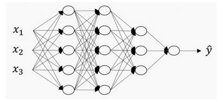
There are 5 neurons in the first layer (the first hidden layer), 5 neurons in the second layer and 3 neurons in the third layer
Represented by symbols, n [ 0 ] = 3 , n [ 1 ] = 5 , n [ 2 ] = 5 , n [ 3 ] = 3 , n [ 4 ] = 1 n^{[0]}=3,n^{[1]}=5,n^{[2]}=5,n^{[3]}=3,n^{[4]}=1 n[0]=3,n[1]=5,n[2]=5,n[3]=3,n[4]=1
For layer i, use a [ i ] a^{[i]} a[i] to represent the result of activation of this layer. The forward part will calculate a [ i ] a^{[i]} a[i]

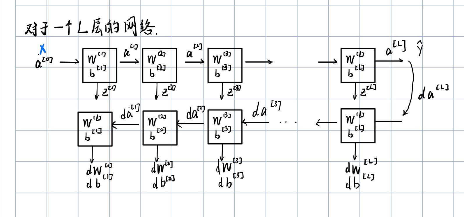
Forward and backward propagation

Forward propagation

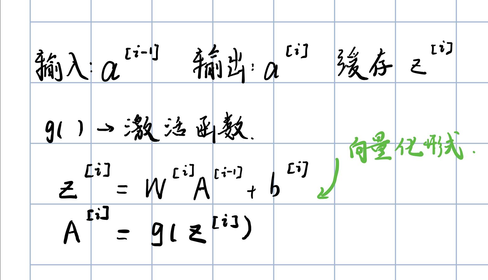
Forward propagation needs to be initialized with X.

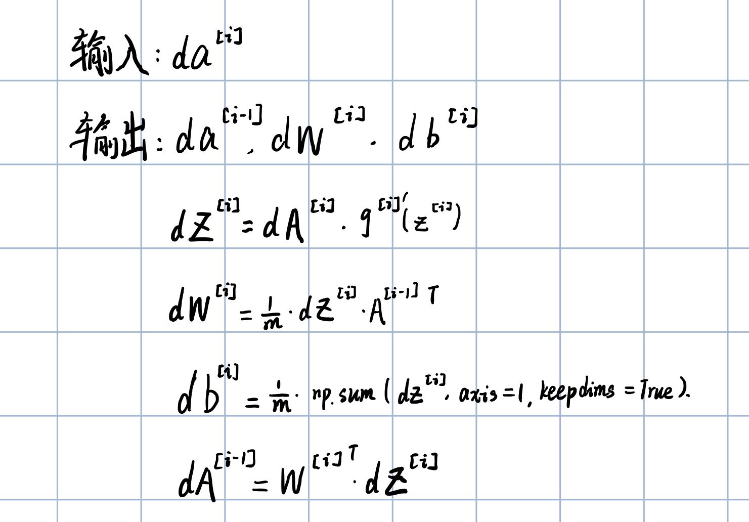
Back propagation

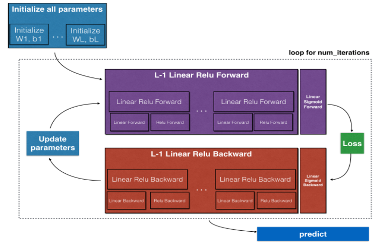
Building neural network blocks

Super parameter

learning rate α \alpha α (learning rate), iterations (number of gradient descent cycles), L (number of hidden layers) n [ l ] n^{[l]} n[l] (number of hidden layer cells), choice of activation function... These parameters control the final W and b

Code operation - helper function

First, you need to introduce related packages

import numpy as np
import h5py
import matplotlib.pyplot as plt
from testCases_v2 import *
from dnn_utils_v2 import sigmoid, sigmoid_backward, relu, relu_backward

%matplotlib inline
plt.rcParams['figure.figsize'] = (5.0, 4.0) # set default size of plots
plt.rcParams['image.interpolation'] = 'nearest'
plt.rcParams['image.cmap'] = 'gray'

%load_ext autoreload
%autoreload 2

np.random.seed(1)

Before building a complete deep neural network, we need to implement some "helper function s"

initialization

For a two-layer neural network

def initialize_parameters(n_x, n_h, n_y):
    """
    Argument:
    n_x -- Enter layer size size of the input layer
    n_h -- Hidden layer size size of the hidden layer
    n_y -- Output layer size size of the output layer
    
    Returns:
    parameters -- python dictionary containing your parameters:
                    W1 -- weight matrix of shape (n_h, n_x)
                    b1 -- bias vector of shape (n_h, 1)
                    W2 -- weight matrix of shape (n_y, n_h)
                    b2 -- bias vector of shape (n_y, 1)
    """
    
    np.random.seed(1)
    
    ### START CODE HERE ### (≈ 4 lines of code)
    # Note that the shape here should be Tuple, and the number of bracket layers should be noted!
    W1 = np.random.randn(n_h,n_x)*0.01
    b1 = np.zeros((n_h,1))
    W2 = np.random.randn(n_y,n_h)*0.01
    b2 = np.zeros((n_y,1))
    ### END CODE HERE ###
    
    assert(W1.shape == (n_h, n_x))
    assert(b1.shape == (n_h, 1))
    assert(W2.shape == (n_y, n_h))
    assert(b2.shape == (n_y, 1))
    
    parameters = {"W1": W1,
                  "b1": b1,
                  "W2": W2,
                  "b2": b2}
    
    return parameters    

Initialize an L-layer neural network

For a multi-layer neural network, the number of layers must match when initializing

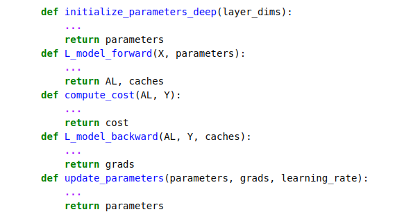
def initialize_parameters_deep(layer_dims):
    """
    Arguments:
    layer_dims -- python array (list) containing the dimensions of each layer in our network
    
    Returns:
    parameters -- python dictionary containing your parameters "W1", "b1", ..., "WL", "bL":
                    Wl -- weight matrix of shape (layer_dims[l], layer_dims[l-1])
                    bl -- bias vector of shape (layer_dims[l], 1)
    """
    
    np.random.seed(3)
    parameters = {}
    L = len(layer_dims)            # number of layers in the network

    for l in range(1, L):
        ### START CODE HERE ### (≈ 2 lines of code)
        parameters['W' + str(l)] = np.random.randn(layer_dims[l], layer_dims[l-1]) * 0.01
        parameters['b' + str(l)] = np.zeros((layer_dims[l], 1))
        ### END CODE HERE ###
        
        assert(parameters['W' + str(l)].shape == (layer_dims[l], layer_dims[l-1]))
        assert(parameters['b' + str(l)].shape == (layer_dims[l], 1))

        
    return parameters

Forward propagation module

Linear Forward

Z [ l ] = W [ l ] A [ l − 1 ] + b [ l ] Z^{[l]}=W^{[l]}A^{[l-1]+b^{[l]}} Z[l]=W[l]A[l − 1]+b[l], where Z [ 0 ] = X Z^{[0]}=X Z[0]=X

def linear_forward(A, W, b):
    """
    Implement the linear part of a layer's forward propagation.

    Arguments:
    A -- activations from previous layer (or input data): (size of previous layer, number of examples)
    W -- weights matrix: numpy array of shape (size of current layer, size of previous layer)
    b -- bias vector, numpy array of shape (size of the current layer, 1)

    Returns:
    Z -- the input of the activation function, also called pre-activation parameter 
    cache -- a python dictionary containing "A", "W" and "b" ; stored for computing the backward pass efficiently
    """
    
    ### START CODE HERE ### (≈ 1 line of code)
    Z = np.dot(W,A)+b
    ### END CODE HERE ###
    
    assert(Z.shape == (W.shape[0], A.shape[1]))
    cache = (A, W, b)
    
    return Z, cache

Linear Forward with activation function

def linear_activation_forward(A_prev, W, b, activation):
    """
    Implement the forward propagation for the LINEAR->ACTIVATION layer

    Arguments:
    A_prev -- activations from previous layer (or input data): (size of previous layer, number of examples)
    W -- weights matrix: numpy array of shape (size of current layer, size of previous layer)
    b -- bias vector, numpy array of shape (size of the current layer, 1)
    activation -- the activation to be used in this layer, stored as a text string: "sigmoid" or "relu"

    Returns:
    A -- the output of the activation function, also called the post-activation value 
    cache -- a python dictionary containing "linear_cache" and "activation_cache";
             stored for computing the backward pass efficiently
    """
    
    if activation == "sigmoid":
        # Inputs: "A_prev, W, b". Outputs: "A, activation_cache".
        ### START CODE HERE ### (≈ 2 lines of code)
        Z, linear_cache = linear_forward(A_prev,W,b)
        A, activation_cache = sigmoid(Z)
        ### END CODE HERE ###
    
    elif activation == "relu":
        # Inputs: "A_prev, W, b". Outputs: "A, activation_cache".
        ### START CODE HERE ### (≈ 2 lines of code)
        Z, linear_cache = linear_forward(A_prev,W,b)
        A, activation_cache = relu(Z)
        ### END CODE HERE ###
    
    assert (A.shape == (W.shape[0], A_prev.shape[1]))
    cache = (linear_cache, activation_cache)

    return A, cache

Forward part of L layer

def L_model_forward(X, parameters):
    """
    Implement forward propagation for the [LINEAR->RELU]*(L-1)->LINEAR->SIGMOID computation
    
    Arguments:
    X -- data, numpy array of shape (input size, number of examples)
    parameters -- output of initialize_parameters_deep()
    
    Returns:
    AL -- last post-activation value
    caches -- list of caches containing:
                every cache of linear_relu_forward() (there are L-1 of them, indexed from 0 to L-2)
                the cache of linear_sigmoid_forward() (there is one, indexed L-1)
    """

    caches = []
    A = X
    L = len(parameters) // 2                  # number of layers in the neural network
    
    # Implement [LINEAR -> RELU]*(L-1). Add "cache" to the "caches" list.
    for l in range(1, L):
        A_prev = A 
         ### START CODE HERE ### (≈ 2 lines of code)
        A, cache = linear_activation_forward(A_prev,parameters['W' + str(l)],parameters['b' + str(l)],activation = "relu")
        caches.append(cache)
        ### END CODE HERE ###
    
    # Implement LINEAR -> SIGMOID. Add "cache" to the "caches" list.
    ### START CODE HERE ### (≈ 2 lines of code)
    AL, cache = linear_activation_forward(A,parameters['W' + str(L)],parameters['b' + str(L)],activation = "sigmoid")
    caches.append(cache)
    ### END CODE HERE ###
    
    assert(AL.shape == (1,X.shape[1]))
            
    return AL, caches

Cost function

The cost function here still uses the formula used before

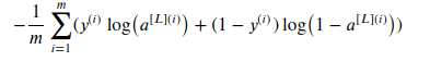
def compute_cost(AL, Y):
    """
    Implement the cost function defined by equation (7).

    Arguments:
    AL -- probability vector corresponding to your label predictions, shape (1, number of examples)
    Y -- true "label" vector (for example: containing 0 if non-cat, 1 if cat), shape (1, number of examples)

    Returns:
    cost -- cross-entropy cost
    """
    
    m = Y.shape[1]

    # Compute loss from aL and y.
    ### START CODE HERE ### (≈ 1 lines of code)
    cost = (-1/m)*np.sum(np.log(AL)*Y+(1-Y)*np.log(1-AL),axis=1,keepdims=True)
    ### END CODE HERE ###
    
    cost = np.squeeze(cost)      # To make sure your cost's shape is what we expect (e.g. this turns [[17]] into 17).
    assert(cost.shape == ())
    
    return cost

Backward part

Linear backward

def linear_backward(dZ, cache):
    """
    Implement the linear portion of backward propagation for a single layer (layer l)

    Arguments:
    dZ -- Gradient of the cost with respect to the linear output (of current layer l)
    cache -- tuple of values (A_prev, W, b) coming from the forward propagation in the current layer

    Returns:
    dA_prev -- Gradient of the cost with respect to the activation (of the previous layer l-1), same shape as A_prev
    dW -- Gradient of the cost with respect to W (current layer l), same shape as W
    db -- Gradient of the cost with respect to b (current layer l), same shape as b
    """
    A_prev, W, b = cache
    m = A_prev.shape[1]
    print(A_prev.shape)
    print(dZ.shape)
    ### START CODE HERE ### (≈ 3 lines of code)
    dW = (1/m)*np.dot(dZ,A_prev.T)
    db = (1/m)*np.sum(dZ,axis=1,keepdims=True)
    dA_prev = W.T*dZ
    ### END CODE HERE ###
    
    assert (dA_prev.shape == A_prev.shape)
    assert (dW.shape == W.shape)
    assert (db.shape == b.shape)
    
    return dA_prev, dW, db

Linear-Activation backward

def linear_activation_backward(dA, cache, activation):
    """
    Implement the backward propagation for the LINEAR->ACTIVATION layer.
    
    Arguments:
    dA -- post-activation gradient for current layer l 
    cache -- tuple of values (linear_cache, activation_cache) we store for computing backward propagation efficiently
    activation -- the activation to be used in this layer, stored as a text string: "sigmoid" or "relu"
    
    Returns:
    dA_prev -- Gradient of the cost with respect to the activation (of the previous layer l-1), same shape as A_prev
    dW -- Gradient of the cost with respect to W (current layer l), same shape as W
    db -- Gradient of the cost with respect to b (current layer l), same shape as b
    """
    linear_cache, activation_cache = cache
    
    if activation == "relu":
        ### START CODE HERE ### (≈ 2 lines of code)
        dZ = relu_backward(dA, activation_cache)
        dA_prev, dW, db = linear_backward(dZ,linear_cache)
        ### END CODE HERE ###
        
    elif activation == "sigmoid":
        ### START CODE HERE ### (≈ 2 lines of code)
        dZ = sigmoid_backward(dA, activation_cache)
        dA_prev, dW, db = linear_backward(dZ,linear_cache)
        ### END CODE HERE ###
    
    return dA_prev, dW, db

backward process of L layer

def L_model_backward(AL, Y, caches):
    """
    Implement the backward propagation for the [LINEAR->RELU] * (L-1) -> LINEAR -> SIGMOID group
    
    Arguments:
    AL -- probability vector, output of the forward propagation (L_model_forward())
    Y -- true "label" vector (containing 0 if non-cat, 1 if cat)
    caches -- list of caches containing:
                every cache of linear_activation_forward() with "relu" (it's caches[l], for l in range(L-1) i.e l = 0...L-2)
                the cache of linear_activation_forward() with "sigmoid" (it's caches[L-1])
    
    Returns:
    grads -- A dictionary with the gradients
             grads["dA" + str(l)] = ...
             grads["dW" + str(l)] = ...
             grads["db" + str(l)] = ...
    """
    grads = {}
    L = len(caches) # the number of layers
    m = AL.shape[1]
    Y = Y.reshape(AL.shape) # after this line, Y is the same shape as AL

    # Initializing the backpropagation
    ### START CODE HERE ### (1 line of code)
    dAL = -(np.divide(Y, AL) - np.divide(1 - Y, 1 - AL))
    ### END CODE HERE ###
    
    # Lth layer (SIGMOID -> LINEAR) gradients. Inputs: "AL, Y, caches". Outputs: "grads["dAL"], grads["dWL"], grads["dbL"]
    ### START CODE HERE ### (approx. 2 lines)
    current_cache = caches[L-1]
    grads["dA" + str(L)], grads["dW" + str(L)], grads["db" + str(L)] = linear_activation_backward(dAL, current_cache, activation="sigmoid")
    ### END CODE HERE 
    
    for l in reversed(range(L - 1)):
        # lth layer: (RELU -> LINEAR) gradients.
        # Inputs: "grads["dA" + str(l + 2)], caches". Outputs: "grads["dA" + str(l + 1)] , grads["dW" + str(l + 1)] , grads["db" + str(l + 1)] 
        ### START CODE HERE ### (approx. 5 lines)
        current_cache = caches[l]
        dA_prev_temp, dW_temp, db_temp = linear_activation_backward(grads["dA" + str(l+2)],current_cache, activation = "relu")
        grads["dA" + str(l + 1)] = dA_prev_temp
        grads["dW" + str(l + 1)] = dW_temp
        grads["db" + str(l + 1)] = db_temp
        ### END CODE HERE ###

    return grads

Parameter update

def update_parameters(parameters, grads, learning_rate):
    """
    Update parameters using gradient descent
    
    Arguments:
    parameters -- python dictionary containing your parameters 
    grads -- python dictionary containing your gradients, output of L_model_backward
    
    Returns:
    parameters -- python dictionary containing your updated parameters 
                  parameters["W" + str(l)] = ... 
                  parameters["b" + str(l)] = ...
    """
    
    L = len(parameters) // 2 # number of layers in the neural network

    # Update rule for each parameter. Use a for loop.
    ### START CODE HERE ### (≈ 3 lines of code)
    for l in range(L):
        parameters["W" + str(l+1)] = parameters["W" + str(l+1)]-learning_rate*grads["dW"+str(l+1)]
        parameters["b" + str(l+1)] = parameters["b" + str(l+1)]-learning_rate*grads["db"+str(l+1)]
    ### END CODE HERE ###
        
    return parameters

Code operation -- implementing neural network

The purpose of this exercise is to use neural network for supervised learning
Or introduce the package first

import time
import numpy as np
import h5py
import matplotlib.pyplot as plt
import scipy
from PIL import Image
from scipy import ndimage
from dnn_app_utils_v2 import *

%matplotlib inline
plt.rcParams['figure.figsize'] = (5.0, 4.0) # set default size of plots
plt.rcParams['image.interpolation'] = 'nearest'
plt.rcParams['image.cmap'] = 'gray'

%load_ext autoreload
%autoreload 2

np.random.seed(1)

Dataset loading

train_x_orig, train_y, test_x_orig, test_y, classes = load_data()

The following code can view the images in the dataset and the number of samples

# Example of a picture
index = 6
plt.imshow(train_x_orig[index])
print ("y = " + str(train_y[0,index]) + ". It's a " + classes[train_y[0,index]].decode("utf-8") +  " picture.")

# Explore your dataset 
m_train = train_x_orig.shape[0]
num_px = train_x_orig.shape[1]
m_test = test_x_orig.shape[0]

print ("Number of training examples: " + str(m_train))
print ("Number of testing examples: " + str(m_test))
print ("Each image is of size: (" + str(num_px) + ", " + str(num_px) + ", 3)")
print ("train_x_orig shape: " + str(train_x_orig.shape))
print ("train_y shape: " + str(train_y.shape))
print ("test_x_orig shape: " + str(test_x_orig.shape))
print ("test_y shape: " + str(test_y.shape))

Before inputting the sample into the neural network, we need to reshape to obtain a feature vector

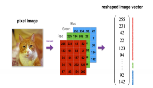
# Reshape the training and test examples 
train_x_flatten = train_x_orig.reshape(train_x_orig.shape[0], -1).T   # The "-1" makes reshape flatten the remaining dimensions
test_x_flatten = test_x_orig.reshape(test_x_orig.shape[0], -1).T

# Standardize data to have feature values between 0 and 1.
train_x = train_x_flatten/255.
test_x = test_x_flatten/255.

print ("train_x's shape: " + str(train_x.shape))
print ("test_x's shape: " + str(test_x.shape))

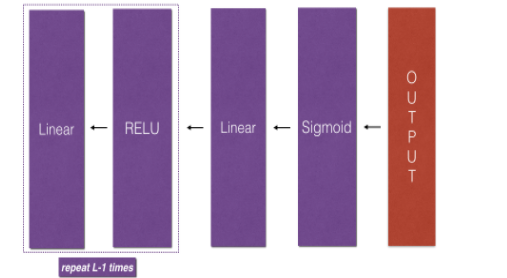
Neural network structure

Layer 2 network (single hidden layer)

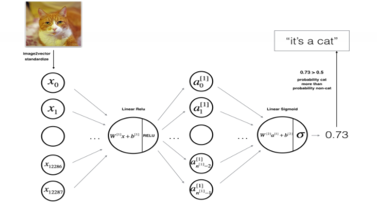
After the feature vector is input, it goes through a linear forward and ReLU activation function, then goes through a linear forward and sigmoid activation function, and finally outputs.

L-layer neural network

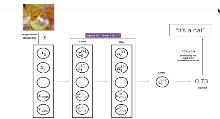
Repeat the linear activation forward in the two-layer neural network L-1 times, and the last time is linear sigmoid forward

Realize two-layer neural network

n_x = 12288     # num_px * num_px * 3
n_h = 7
n_y = 1
layers_dims = (n_x, n_h, n_y)

def two_layer_model(X, Y, layers_dims, learning_rate = 0.0075, num_iterations = 3000, print_cost=False):
    """
    Implements a two-layer neural network: LINEAR->RELU->LINEAR->SIGMOID.
    
    Arguments:
    X -- input data, of shape (n_x, number of examples)
    Y -- true "label" vector (containing 0 if cat, 1 if non-cat), of shape (1, number of examples)
    layers_dims -- dimensions of the layers (n_x, n_h, n_y)
    num_iterations -- number of iterations of the optimization loop
    learning_rate -- learning rate of the gradient descent update rule
    print_cost -- If set to True, this will print the cost every 100 iterations 
    
    Returns:
    parameters -- a dictionary containing W1, W2, b1, and b2
    """
    
    np.random.seed(1)
    grads = {}
    costs = []                              # to keep track of the cost
    m = X.shape[1]                           # number of examples
    (n_x, n_h, n_y) = layers_dims
    
    # Initialize parameters dictionary, by calling one of the functions you'd previously implemented
    ### START CODE HERE ### (≈ 1 line of code)
    parameters = initialize_parameters(n_x, n_h, n_y)
    ### END CODE HERE ###
    
    # Get W1, b1, W2 and b2 from the dictionary parameters.
    W1 = parameters["W1"]
    b1 = parameters["b1"]
    W2 = parameters["W2"]
    b2 = parameters["b2"]
    
    # Loop (gradient descent)

    for i in range(0, num_iterations):

        # Forward propagation: LINEAR -> RELU -> LINEAR -> SIGMOID. Inputs: "X, W1, b1". Output: "A1, cache1, A2, cache2".
        ### START CODE HERE ### (≈ 2 lines of code)
        A1, cache1 = linear_activation_forward(X, W1, b1, activation="relu")
        A2, cache2 = linear_activation_forward(A1, W2, b2, activation="sigmoid")
        ### END CODE HERE ###
        
        # Compute cost
        ### START CODE HERE ### (≈ 1 line of code)
        cost = compute_cost(A2, Y)
        ### END CODE HERE ###
        
        # Initializing backward propagation
        dA2 = - (np.divide(Y, A2) - np.divide(1 - Y, 1 - A2))
        
        # Backward propagation. Inputs: "dA2, cache2, cache1". Outputs: "dA1, dW2, db2; also dA0 (not used), dW1, db1".
        ### START CODE HERE ### (≈ 2 lines of code)
        dA1, dW2, db2 = linear_activation_backward(dA2, cache2, activation="sigmoid")
        dA0, dW1, db1 = linear_activation_backward(dA1, cache1, activation="relu")
        ### END CODE HERE ###
        
        # Set grads['dWl'] to dW1, grads['db1'] to db1, grads['dW2'] to dW2, grads['db2'] to db2
        grads['dW1'] = dW1
        grads['db1'] = db1
        grads['dW2'] = dW2
        grads['db2'] = db2
        
        # Update parameters.
        ### START CODE HERE ### (approx. 1 line of code)
        parameters = update_parameters(parameters, grads, learning_rate=0.0075)
        ### END CODE HERE ###

        # Retrieve W1, b1, W2, b2 from parameters
        W1 = parameters["W1"]
        b1 = parameters["b1"]
        W2 = parameters["W2"]
        b2 = parameters["b2"]
        
        # Print the cost every 100 training example
        if print_cost and i % 100 == 0:
            print("Cost after iteration {}: {}".format(i, np.squeeze(cost)))
        if print_cost and i % 100 == 0:
            costs.append(cost)
       
    # plot the cost

    plt.plot(np.squeeze(costs))
    plt.ylabel('cost')
    plt.xlabel('iterations (per tens)')
    plt.title("Learning rate =" + str(learning_rate))
    plt.show()
    
    return parameters

Call as follows

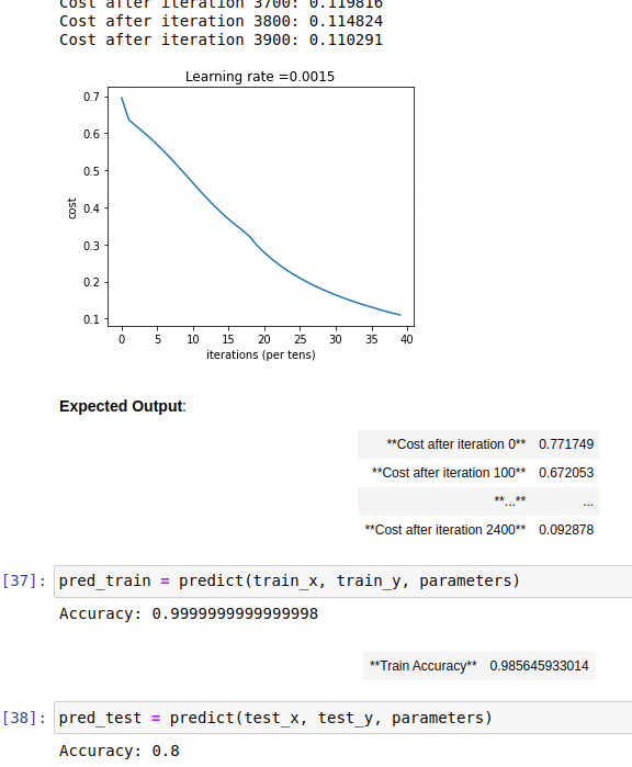
parameters = two_layer_model(train_x, train_y, layers_dims = (n_x, n_h, n_y), num_iterations = 2500, print_cost=True)

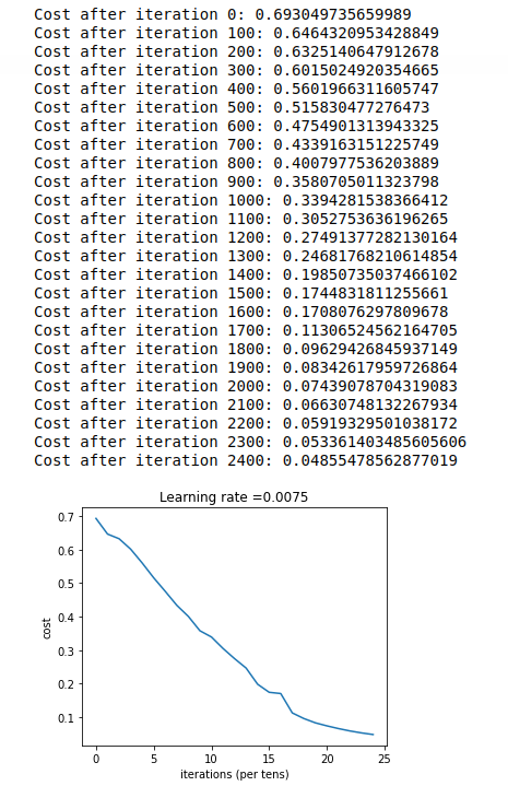
The accuracy rate of two-layer network is 72%, which is similar to that of logistic regression. However, increasing the number of network layers may improve the accuracy rate.

Realize L-layer neural network

Before starting to build the L-layer neural network, list the possible help function s

Here we will build a five layer neural network

layers_dims = [12288, 20, 7, 5, 1] #  5-layer model

def L_layer_model(X, Y, layers_dims, learning_rate = 0.0075, num_iterations = 3000, print_cost=False):#lr was 0.009
    """
    Implements a L-layer neural network: [LINEAR->RELU]*(L-1)->LINEAR->SIGMOID.
    
    Arguments:
    X -- data, numpy array of shape (number of examples, num_px * num_px * 3)
    Y -- true "label" vector (containing 0 if cat, 1 if non-cat), of shape (1, number of examples)
    layers_dims -- list containing the input size and each layer size, of length (number of layers + 1).
    learning_rate -- learning rate of the gradient descent update rule
    num_iterations -- number of iterations of the optimization loop
    print_cost -- if True, it prints the cost every 100 steps
    
    Returns:
    parameters -- parameters learnt by the model. They can then be used to predict.
    """

    np.random.seed(1)
    costs = []                         # keep track of cost
    
    # Parameters initialization.
    ### START CODE HERE ###
    parameters = initialize_parameters_deep(layers_dims)
    ### END CODE HERE ###
    
    # Loop (gradient descent)
    for i in range(0, num_iterations):

        # Forward propagation: [LINEAR -> RELU]*(L-1) -> LINEAR -> SIGMOID.
        ### START CODE HERE ### (≈ 1 line of code)
        AL, caches =  L_model_forward(X, parameters)
        ### END CODE HERE ###
        
        # Compute cost.
        ### START CODE HERE ### (≈ 1 line of code)
        cost = compute_cost(AL, Y)
        ### END CODE HERE ###
    
        # Backward propagation.
        ### START CODE HERE ### (≈ 1 line of code)
        grads = L_model_backward(AL, Y, caches)
        ### END CODE HERE ###
 
        # Update parameters.
        ### START CODE HERE ### (≈ 1 line of code)
        parameters = update_parameters(parameters, grads, learning_rate=0.0075)
        ### END CODE HERE ###
                
        # Print the cost every 100 training example
        if print_cost and i % 100 == 0:
            print ("Cost after iteration %i: %f" %(i, cost))
        if print_cost and i % 100 == 0:
            costs.append(cost)
            
    # plot the cost
    plt.plot(np.squeeze(costs))
    plt.ylabel('cost')
    plt.xlabel('iterations (per tens)')
    plt.title("Learning rate =" + str(learning_rate))
    plt.show()
    
    return parameters

Problems encountered

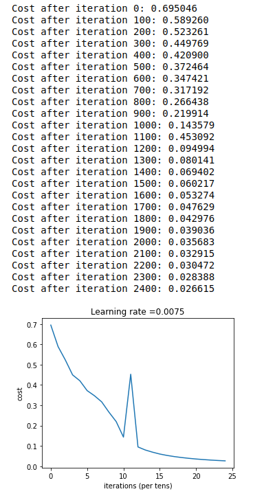
The above image is obviously wrong. Facts have proved that its accuracy is 74%, which is not so much higher than that of logistic regression.
Then learn the learning rate_ When the rate is set to 0.0015, the accuracy of the test set is increased to 80%