1-packges

Before we start, we need to import the following libraries:

• numpy: it is a basic software package for scientific computing in Python.
• h5py: a common software package that interacts with data sets stored in H5 files.
• matplotlib: is a well-known library for drawing charts in Python.
• lr_utils: in the package of this article, a library of simple functions to load the data in the package.

import numpy as np
import copy
import matplotlib.pyplot as plt
import h5py
import scipy
from PIL import Image
from scipy import ndimage
from lr_utils import load_dataset
from public_tests import *

%matplotlib inline
%load_ext autoreload
%autoreload 2

2- Overview of the Problem set

Problem statement: there is a training set and test set, in which there are data marked as cat and non cat, so we want to build a simple image recognition algorithm.

Load data

# Loading the data (cat/non-cat)
train_set_x_orig, train_set_y, test_set_x_orig, test_set_y, classes = load_dataset()

"_orig" is added at the end of the image data set (training and testing) to preprocess them.
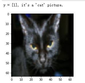
Let's take a random look at the pictures in the training set.

# Example of a picture
index = 25
plt.imshow(train_set_x_orig[index])
print ("y = " + str(train_set_y[:, index]) + ", it's a '" + classes[np.squeeze(train_set_y[:, index])].decode("utf-8") +  "' picture.")

The output result is

2-1 Exercise 1

Known dataset parameters:

• m_train: the number of pictures in the training set.
• m_test: the number of pictures in the test set.
• num_px: width and height of pictures in training and test sets (both 64x64)

Tips:
train_set_x_orig is an array with dimension (m_train, num_px, num_px, 3).
You can get m_train through train_set_x_orig.shape[0].

#(≈ 3 lines of code)
# m_train = 
# m_test = 
# num_px = 
# YOUR CODE STARTS HERE
m_train = train_set_x_orig.shape[0]
m_test = test_set_x_orig.shape[0]
num_px = train_set_x_orig.shape[1] 

# YOUR CODE ENDS HERE

print ("Number of training examples: m_train = " + str(m_train))
print ("Number of testing examples: m_test = " + str(m_test))
print ("Height/Width of each image: num_px = " + str(num_px))
print ("Each image is of size: (" + str(num_px) + ", " + str(num_px) + ", 3)")
print ("train_set_x shape: " + str(train_set_x_orig.shape))
print ("train_set_y shape: " + str(train_set_y.shape))
print ("test_set_x shape: " + str(test_set_x_orig.shape))
print ("test_set_y shape: " + str(test_set_y.shape))

Output results

2-2 Exercise 2

Tile the training set and test set array with dimension (num_px, num_px, 3) as (num_px * num_px * 3, 1).
Tips:
When you want to tile matrix X of shape (a, B, C, d) into matrix x_flat of shape (b * c * d, a), you can use the following code:

X_flatten = X.reshape(X.shape[0], -1).T      # X.T is the transpose of X
#reshape(m,-1) changes the dimension to M rows and d columns, - 1 indicates that the number of columns is calculated automatically

So there

# Reshape the training and test examples
#(≈ 2 lines of code)
# train_set_x_flatten = ...
# test_set_x_flatten = ...
# YOUR CODE STARTS HERE
train_set_x_flatten = train_set_x_orig.reshape(train_set_x_orig.shape[0],-1).T
test_set_x_flatten = test_set_x_orig.reshape(test_set_x_orig.shape[0],-1).T

# YOUR CODE ENDS HERE

# Check that the first 10 pixels of the second image are in the correct place
assert np.alltrue(train_set_x_flatten[0:10, 1] == [196, 192, 190, 193, 186, 182, 188, 179, 174, 213]), "Wrong solution. Use (X.shape[0], -1).T."
assert np.alltrue(test_set_x_flatten[0:10, 1] == [115, 110, 111, 137, 129, 129, 155, 146, 145, 159]), "Wrong solution. Use (X.shape[0], -1).T."

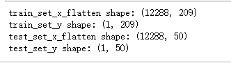
print ("train_set_x_flatten shape: " + str(train_set_x_flatten.shape))
print ("train_set_y shape: " + str(train_set_y.shape))
print ("test_set_x_flatten shape: " + str(test_set_x_flatten.shape))
print ("test_set_y shape: " + str(test_set_y.shape))

output

To represent a color image, you must specify red, green, and blue channels (RGB) for each pixel Therefore, the pixel value is actually a vector of three numbers in the range from 0 to 255. A common preprocessing step in machine learning is to center and standardize the data set, which means that the average value of the whole numpy array in each example can be subtracted, and then each example can be divided by the standard deviation of the whole numpy array. However, for image data sets, it is simpler and more convenient , almost every row of the dataset can be divided by 255 (the maximum value of the pixel channel). Because there is no data larger than 255 in RGB, we can safely divide by 255 to make the standardized data between [0,1]. Now standardize our dataset:

train_set_x = train_set_x_flatten / 255.
test_set_x = test_set_x_flatten / 255.

Common steps for preprocessing a new dataset are:
1. Find out the size and shape of the problem (m_train, m_test, num_px,...)
2. Reshape the dataset so that each example is now a vector of size (num_px * num_px * 3,1).
3. "Standardized" data

3 - General Architecture of the learning algorithm

Next, we need to design a simple algorithm, using the neural network of logistic regression.

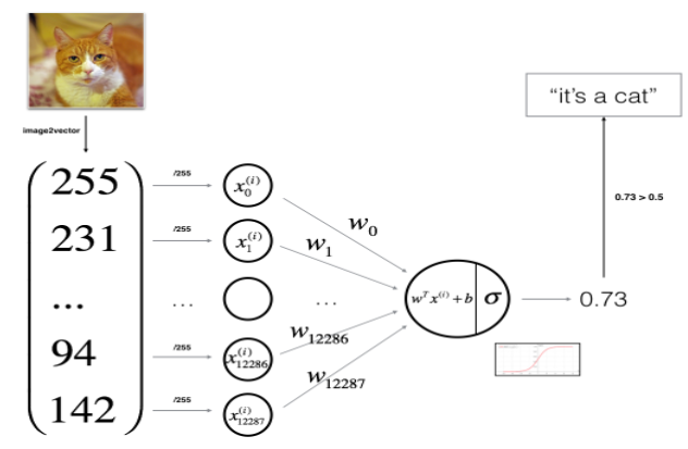
Mathematical expression:

4 - Building the parts of our algorithm

The main steps of establishing neural network are:

1. Define the structure of the model (for example, the number of input features)

2. Initialize the parameters of the model

3. Cycle:

3.1 calculation of current loss (forward propagation)

3.2 calculate current gradient (back propagation)

3.3 update parameters (gradient descent)

4.1 - Helper functions- Exercise 3

Build sigmoid().

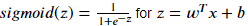
# GRADED FUNCTION: sigmoid

def sigmoid(z):
    """
    Compute the sigmoid of z

    Arguments:
    z -- Scalar or of any size numpy Array.

    Return:
    s -- sigmoid(z)
    """

    #(≈ 1 line of code)
    # s = ...
    # YOUR CODE STARTS HERE
    s = 1 / (1 + np.exp(-z))
    
    # YOUR CODE ENDS HERE
    
    return s

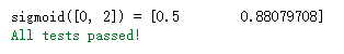
Let's test the sigmoid() function

print ("sigmoid([0, 2]) = " + str(sigmoid(np.array([0,2]))))
#The outputs are sigmoid(0) and sigmoid(2) respectively
sigmoid_test(sigmoid)

x = np.array([0.5, 0, 2.0])
output = sigmoid(x)
print(output)

4.2 - Initializing parameters- Exercise 4

Implement parameter initialization

Tips
Use np.zeros(). Return an array filled with 0 for the given shape and type.

def initialize_with_zeros(dim):
    """
        This function is w Create a dimension for( dim，1)0 vector, and b Initialize to 0.
        
        Parameters:
            dim  - What we want w The size of the vector (or the number of parameters in this case)
        
        return:
            w  - Dimension is( dim，1)Initialization vector for.
            b  - Initialized scalar (corresponding to deviation)
    """
    w = np.zeros(shape = (dim,1))
    b = float(0) #Note that this place must be defined as floating point, otherwise an error will be reported
    #Use assertions to ensure that the data I want is correct
    assert(w.shape == (dim, 1)) #The dimension of w is (dim,1)
    assert(isinstance(b, float) or isinstance(b, int)) #The type of b is float or int
    
    return (w , b)

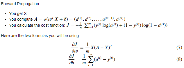
4.3 - Forward and Backward propagation- Exercise 5

You can now perform forward / backward propagation steps to learn parameters.
First, we need to implement a cost function and its gradient function, propagate ().
Tips:

Tips
Use np.log() and np.dot() [(multiplication of two matrices)] and np.sum() [can be used to calculate the accumulation of i].

def propagate(w, b, X, Y):
	"""
    Realize the cost function and its gradient of forward and backward propagation.
    Parameters:
        w  - Weights, arrays of different sizes( num_px * num_px * 3，1)
        b  - Deviation, a scalar
        X  - Matrix type is( num_px * num_px * 3，Training quantity)
        Y  - True label vector (0 if non cat, 1 if cat), matrix dimension(1,Number of training data)

    return:
        cost- Negative log likelihood cost of logistic regression
        dw  - be relative to w The loss gradient is therefore associated with w Same shape
        db  - be relative to b The loss gradient is therefore associated with b The shape of the is the same
    """
	m = X.shape[1]
    
    #Forward propagation
    A = sigmoid(np.dot(w.T,X) + b) #To calculate the activation value, refer to formula 2.
    cost = (- 1 / m) * np.sum(Y * np.log(A) + (1 - Y) * (np.log(1 - A))) #For cost calculation, please refer to formulas 3 and 4.
    
    #Back propagation
    dw = (1 / m) * np.dot(X, (A - Y).T) #Please refer to the partial derivative formula in the video.
    db = (1 / m) * np.sum(A - Y) #Please refer to the partial derivative formula in the video.
	
	#Use assertions to ensure that my data is correct
    assert(dw.shape == w.shape)
    assert(db.dtype == float)
    cost = np.squeeze(cost)
    assert(cost.shape == ())
    
    #Create a dictionary and save dw and db.
    grads = {
                "dw": dw,
                "db": db
             }
    return (grads , cost)

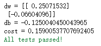
Then test

w =  np.array([[1.], [2]])
b = 1.5
X = np.array([[1., -2., -1.], [3., 0.5, -3.2]])
Y = np.array([[1, 1, 0]])
grads, cost = propagate(w, b, X, Y)

assert type(grads["dw"]) == np.ndarray
assert grads["dw"].shape == (2, 1)
assert type(grads["db"]) == np.float64


print ("dw = " + str(grads["dw"]))
print ("db = " + str(grads["db"]))
print ("cost = " + str(cost))

propagate_test(propagate)

Output as

4.4 - Optimization- Exercise 6

Use gradient descent to update parameters.
The goal is to learn w and b by minimizing the cost function J θ \theta θ The update rule for is θ = θ − α d ( θ ) \theta = \theta-\alpha d( \theta ) θ=θ − α d( θ). among α \alpha α Is the learning rate.

# GRADED FUNCTION: optimize

def optimize(w, b, X, Y, num_iterations=100, learning_rate=0.009, print_cost=False):
    """
    This function is optimized by running the gradient descent algorithm w and b
    
    Parameters:
        w  - Weights, arrays of different sizes( num_px * num_px * 3，1)
        b  - Deviation, a scalar
        X  - Dimension is( num_px * num_px * 3，An array of training data.
        Y  - True label vector (0 if non cat, 1 if cat), matrix dimension(1,Number of training data)
        num_iterations  - Number of iterations of the optimization cycle
        learning_rate  - Learning rate of gradient descent update rule
        print_cost  - Print the loss value every 100 steps
    
    return:
        params  - Include weight w And deviation b Dictionary of
        grads  - A dictionary containing gradients of weights and deviations relative to the cost function
        cost - A list of all costs calculated during optimization will be used to draw the learning curve.
    
    Tips:
    We need to write down the following two steps and traverse them:
        1)Calculate the cost and gradient of the current parameter, using propagate(). 
        2)use w and b The gradient descent rule updates the parameters.

    """
    
    w = copy.deepcopy(w)
    b = copy.deepcopy(b)
    
    costs = []
    
    for i in range(num_iterations):
        # (≈ 1 lines of code)
        # Cost and gradient calculation 
        # grads, cost = ...
        # YOUR CODE STARTS HERE
        grads, cost =   propagate(w, b, X, Y)     

        
        # YOUR CODE ENDS HERE
        
        # Retrieve derivatives from grads
        dw = grads["dw"]
        db = grads["db"]
        
        # update rule (≈ 2 lines of code)
        # w = ...
        # b = ...
        # YOUR CODE STARTS HERE
        w = w - learning_rate* dw
        b = b - learning_rate * db
        
        # YOUR CODE ENDS HERE
        
        # Record the costs
        if i % 100 == 0:
            costs.append(cost)
        
            # Print the cost every 100 training iterations
            if print_cost:
                print ("Cost after iteration %i: %f" %(i, cost))
    
    params = {"w": w,
              "b": b}
    
    grads = {"dw": dw,
             "db": db}
    
    return params, grads, costs

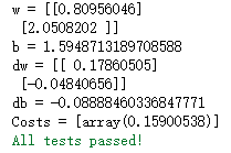
Test optimization function:

params, grads, costs = optimize(w, b, X, Y, num_iterations=100, learning_rate=0.009, print_cost=False)

print ("w = " + str(params["w"]))
print ("b = " + str(params["b"]))
print ("dw = " + str(grads["dw"]))
print ("db = " + str(grads["db"]))
print("Costs = " + str(costs))

optimize_test(optimize)

output

4.4 - Optimization- Exercise 7

The optimize function will output the learned values of W and b. we can use w and b to predict the label of dataset X. now we want to implement the prediction function predict(). There are two steps to calculate the prediction:

# GRADED FUNCTION: predict

def predict(w, b, X):
    '''
   Using learning logistic regression parameters logistic (w，b)Whether the forecast tag is 0 or 1,
    
    Parameters:
        w  - Weights, arrays of different sizes( num_px * num_px * 3，1)
        b  - Deviation, a scalar
        X  - Dimension is( num_px * num_px * 3，Number of training data)
    
    return:
        Y_prediction  - contain X All predictions for all pictures in [0] | 1]One of numpy Array (vector)
    '''
    
    m = X.shape[1] #Number of pictures
    Y_prediction = np.zeros((1, m))
    w = w.reshape(X.shape[0], 1)
    
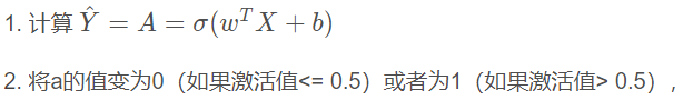
    # Calculate A and predict the probability of cats appearing in the picture
    #(≈ 1 line of code)
    # A = ...
    # YOUR CODE STARTS HERE
    A = sigmoid(np.dot(w.T , X) + b)
    
    # YOUR CODE ENDS HERE
    
    for i in range(A.shape[1]):
        
        # Convert probabilities A[0,i] to actual predictions p[0,i]
        #(≈ 4 lines of code)
        # if A[0, i] > ____ :
        #     Y_prediction[0,i] = 
        # else:
        #     Y_prediction[0,i] = 
        # YOUR CODE STARTS HERE
        if A[0, i] > 0.5 :
             Y_prediction[0,i] = 1 
        else:
            Y_prediction[0,i] = 0 
        
        # YOUR CODE ENDS HERE
    
    return Y_prediction

test

w = np.array([[0.1124579], [0.23106775]])
b = -0.3
X = np.array([[1., -1.1, -3.2],[1.2, 2., 0.1]])
print ("predictions = " + str(predict(w, b, X)))

predict_test(predict)

result

5 - Merge all functions into a model - Exercise 8

Integrate these functions into a model() function.

def model(X_train , Y_train , X_test , Y_test , num_iterations = 2000 , learning_rate = 0.5 , print_cost = False):
    """
    Build the logistic regression model by calling the previously implemented functions
    
    Parameters:
        X_train  - numpy Array of,Dimension is( num_px * num_px * 3，m_train)Training set for
        Y_train  - numpy Array of,Dimension is (1, m_train)(Training label set for vector)
        X_test   - numpy Array of,Dimension is( num_px * num_px * 3，m_test)Test set for
        Y_test   - numpy Array of,Dimension is (1, m_test)Set of test tags for (vector)
        num_iterations  - A hyperparameter that represents the number of iterations used to optimize the parameter
        learning_rate  - express optimize()Update the superparameter of the learning rate used in the rule
        print_cost  - Set to true Print cost per 100 iterations
    
    return:
        d  - A dictionary that contains information about the model.
    """
    w , b = initialize_with_zeros(X_train.shape[0])
    
    parameters , grads , costs = optimize(w , b , X_train , Y_train,num_iterations , learning_rate , print_cost)
    
    #Retrieve parameters w and b from the dictionary parameters
    w , b = parameters["w"] , parameters["b"]
    
    #Examples of predictive test / training sets
    Y_prediction_test = predict(w , b, X_test)
    Y_prediction_train = predict(w , b, X_train)
    
    #Print accuracy after training
    print("Training set accuracy:"  , format(100 - np.mean(np.abs(Y_prediction_train - Y_train)) * 100) ,"%")
    print("Test set accuracy:"  , format(100 - np.mean(np.abs(Y_prediction_test - Y_test)) * 100) ,"%")
    
    d = {
            "costs" : costs,
            "Y_prediction_test" : Y_prediction_test,
            "Y_prediciton_train" : Y_prediction_train,
            "w" : w,
            "b" : b,
            "learning_rate" : learning_rate,
            "num_iterations" : num_iterations }
    return d

Finally, test

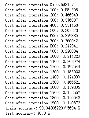
logistic_regression_model = model(train_set_x, train_set_y, test_set_x, test_set_y, num_iterations=2000, learning_rate=0.005, print_cost=True)

Result (number of iterations: error value)

Examples of image classification errors

index = 1
plt.imshow(test_set_x[:, index].reshape((num_px, num_px, 3)))
print ("y = " + str(test_set_y[0,index]) + ", you predicted that it is a \"" + classes[int(logistic_regression_model['Y_prediction_test'][0,index])].decode("utf-8") +  "\" picture.")