Recently, when writing a paper, I encountered the problem of feature graph visualization, so I sorted the methods to solve this problem into notes.

1: Why visualization?

It is often said that the essence of CNN is to extract features, but we don't know what features it extracts, which regions really play a role in recognition, or what the network obtains the classification results. At this time, we analyze its shortcomings according to the results of visualizing a network, so as to put forward new improvement methods.

2: CNN visualization method

① : feature map visualization. There are two methods for feature graph visualization. One is to directly map the feature map of a layer to the range of 0-255 and turn it into an image. The other is to use a deconvolution network (deconvolution and de pooling) to turn the feature map into an image, so as to achieve the purpose of visualizing the feature map.

② : convolution kernel visualization.

③ : class activates visualization. This is mainly used to determine which areas of the image play a major role in identifying a class. Such as the common Heat Map, when recognizing cats, the Heat Map can directly see the effect of each area in the image on identifying cats. At present, the main methods used are cam series (CAM, grad cam, grad cam + +).

④ : some technical tools. A certain layer of CNN model is visualized by some researchers' open source tools.

The above four methods are described in detail by the boss. You can take a look if necessary: Reference 1

3: YOLOV5 feature map visualization

The following figure shows the best you have trained The characteristic diagram of the first Focus module after visualization during Pt detect:

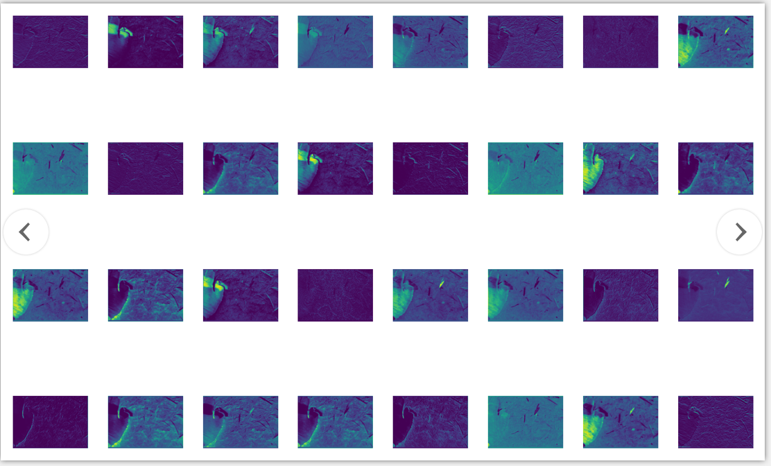
It can be seen that the features extracted from different feature maps are almost different. Some Focus on the edge, while others Focus on the whole. Of course, this is only the first Focus feature map. Compared with the deeper features, the shallow features are mostly complete, while the deeper features are smaller, and they are small features extracted. Of course, These characteristic graphs are also interrelated, and the network structure is a whole.

yolov5 what the author said in issue:

BTW, a single feature map may be in my opinion a shallow set of information, as you are looking at a 2d spatial slice but are not aptly observing relationships across the feature space (as the convolutions do).

I guess an analogy is that you would be viewing the R, G, B layers of a color image by themselves, when it helps to view them together to get the complete picture.

3.1 code implementation

(1) Changes in the code

General. In utils is required Py or plots Py add the following functions:

import matplotlib.pyplot as plt
from torchvision import transforms
 
 
def feature_visualization(features, model_type, model_id, feature_num=64):
    """
    features: The feature map which you need to visualization
    model_type: The type of feature map
    model_id: The id of feature map
    feature_num: The amount of visualization you need
    """
    save_dir = "features/"
    if not os.path.exists(save_dir):
        os.makedirs(save_dir)
 
    # print(features.shape)
    # block by channel dimension
    blocks = torch.chunk(features, features.shape[1], dim=1)
 
    # # size of feature
    # size = features.shape[2], features.shape[3]
 
    plt.figure()
    for i in range(feature_num):
        torch.squeeze(blocks[i])
        feature = transforms.ToPILImage()(blocks[i].squeeze())
        # print(feature)
        ax = plt.subplot(int(math.sqrt(feature_num)), int(math.sqrt(feature_num)), i+1)
        ax.set_xticks([])
        ax.set_yticks([])
 
        plt.imshow(feature)
        # gray feature
        # plt.imshow(feature, cmap='gray')
 
    # plt.show()
    plt.savefig(save_dir + '{}_{}_feature_map_{}.png'
                .format(model_type.split('.')[2], model_id, feature_num), dpi=300)

Then, in models, Yolo Py, add the following code:

    def forward_once(self, x, profile=False):
        y, dt = [], []  # outputs
        for m in self.model:
            if m.f != -1:  # if not from previous layer
                x = y[m.f] if isinstance(m.f, int) else [x if j == -1 else y[j] for j in m.f]  # from earlier layers

            if profile:
                o = thop.profile(m, inputs=(x,), verbose=False)[0] / 1E9 * 2 if thop else 0  # FLOPS
                t = time_synchronized()
                for _ in range(10):
                    _ = m(x)
                dt.append((time_synchronized() - t) * 100)
                print('%10.1f%10.0f%10.1fms %-40s' % (o, m.np, dt[-1], m.type))

            x = m(x)  # run
            y.append(x if m.i in self.save else None)  # save output
            # Feature map visualization added here
            '''
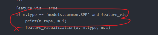
            feature_vis = True
            if m.type == 'models.common.SPP' and feature_vis:
                print(m.type, m.i)
                feature_visualization(x, m.type, m.i)           
           
            '''
        if profile:
            print('%.1fms total' % sum(dt))

And in Yolo Add the following functions at the beginning of Py:

from utils.general import feature_visualization

(2) Pay attention

① : one thing to note:

yolov5 will first summarize the model in the process of detect ing or train ing, that is, verify the layers, parameters and gradients of your model. This process will also save the feature map, but don't worry, because the saved feature map name is the same and will be overwritten. If you print out the log, you will see that the whole model runs twice.

Model Summary: 224 layers, 7056607 parameters, 0 gradients

② : if you want the feature map of a structure, you can modify it in this place

For example, output the characteristic diagram of the last three detection layers (i.e. layers 17, 20 and 23 in the configuration file)

Put this line of code
if m.type == 'models.common.C3' and feature_vis:
Replace with
if m.i=='17, 20, 23' and feature_vis:

Reference 2

③ : the latest yolov5 version on GitHub already has visual code. You can download the latest version for verification.

python detect.py --weights runs/exp/weights/best.pt

Just run the above code.

In Xiaobai's study, this note is purely for study. If there is infringement, please contact me to delete it