In object detection, due to the limitations of cost and application occasions, we can't blindly increase the resolution of the camera, or we have used a camera with high resolution, but the field of view is large and still can't achieve high accuracy. At this time, we should consider sub-pixel technology, which is to further subdivide between two pixels, So as to obtain the coordinates of sub-pixel edge points (that is, the coordinates of float type). Generally speaking, the existing technology can achieve 2 subdivision, 4 subdivision, or even higher. Through the use of sub-pixel edge detection technology, the cost can be saved and the recognition accuracy can be improved.

Common sub-pixel technologies include gray moment, Hu moment, spatial moment, Zernike moment, etc. by consulting several papers and comprehensively comparing the accuracy, time and implementation difficulty, Zernike moment is selected as the sub-pixel edge detection algorithm in the project. Based on the edge detection principle of Zernike moment, the next article will summarize it in detail. Here, the steps are generally described and implemented by OpenCV.

The general step is to first determine the size of the template used, and then calculate the coefficients of each template according to the formula of Zernike moment. For example, I choose 7 * 7 template (the larger the template, the higher the accuracy, but the longer the operation time). To calculate M00, M11R, M11I, M20, M31R, M31I and M40 seven Zernike templates. The second step is to preprocess the image to be detected, including filtering binarization, or Canny edge detection. The third step is to convolute the preprocessed image with seven Zernike moment templates to obtain seven Zernike moments. The fourth step is to multiply the moment of the previous step by the angle correction coefficient (this is because using Zernike's rotation invariance, Zernike model simplifies the edges into a straight line with x=n, which should be adjusted here). The fifth step is to calculate the distance parameter l and the gray difference parameter k, and judge whether the point is an edge point according to k and l. The following is the implementation based on OpenCV.

For the theoretical part, please refer to: (12 messages) edge detection of zernike moment (with source code)_ xiaoluo91's column - CSDN blog_ zernike moment edge detection

The following part is the code snippet of python implementation, which is for reference only.

import cv2
import numpy as np
import matplotlib.pyplot as plt
import time

g_N = 7

M00 = np.array([0, 0.0287, 0.0686, 0.0807, 0.0686, 0.0287, 0,
	0.0287, 0.0815, 0.0816, 0.0816, 0.0816, 0.0815, 0.0287,
	0.0686, 0.0816, 0.0816, 0.0816, 0.0816, 0.0816, 0.0686,
	0.0807, 0.0816, 0.0816, 0.0816, 0.0816, 0.0816, 0.0807,
	0.0686, 0.0816, 0.0816, 0.0816, 0.0816, 0.0816, 0.0686,
	0.0287, 0.0815, 0.0816, 0.0816, 0.0816, 0.0815, 0.0287,
	0, 0.0287, 0.0686, 0.0807, 0.0686, 0.0287, 0]).reshape((7, 7))


M11R = np.array([0, -0.015, -0.019, 0, 0.019, 0.015, 0,
	-0.0224, -0.0466, -0.0233, 0, 0.0233, 0.0466, 0.0224,
	-0.0573, -0.0466, -0.0233, 0, 0.0233, 0.0466, 0.0573,
	-0.069, -0.0466, -0.0233, 0, 0.0233, 0.0466, 0.069,
	-0.0573, -0.0466, -0.0233, 0, 0.0233, 0.0466, 0.0573,
	-0.0224, -0.0466, -0.0233, 0, 0.0233, 0.0466, 0.0224,
	0, -0.015, -0.019, 0, 0.019, 0.015, 0]).reshape((7, 7))


M11I = np.array([0, -0.0224, -0.0573, -0.069, -0.0573, -0.0224, 0,
	-0.015, -0.0466, -0.0466, -0.0466, -0.0466, -0.0466, -0.015,
	-0.019, -0.0233, -0.0233, -0.0233, -0.0233, -0.0233, -0.019,
	0, 0, 0, 0, 0, 0, 0,
	0.019, 0.0233, 0.0233, 0.0233, 0.0233, 0.0233, 0.019,
	0.015, 0.0466, 0.0466, 0.0466, 0.0466, 0.0466, 0.015,
	0, 0.0224, 0.0573, 0.069, 0.0573, 0.0224, 0]).reshape((7, 7))


M20 = np.array([0, 0.0225, 0.0394, 0.0396, 0.0394, 0.0225, 0,
	0.0225, 0.0271, -0.0128, -0.0261, -0.0128, 0.0271, 0.0225,
	0.0394, -0.0128, -0.0528, -0.0661, -0.0528, -0.0128, 0.0394,
	0.0396, -0.0261, -0.0661, -0.0794, -0.0661, -0.0261, 0.0396,
	0.0394, -0.0128, -0.0528, -0.0661, -0.0528, -0.0128, 0.0394,
	0.0225, 0.0271, -0.0128, -0.0261, -0.0128, 0.0271, 0.0225,
	0, 0.0225, 0.0394, 0.0396, 0.0394, 0.0225, 0]).reshape((7, 7))


M31R = np.array([0, -0.0103, -0.0073, 0, 0.0073, 0.0103, 0,
	-0.0153, -0.0018, 0.0162, 0, -0.0162, 0.0018, 0.0153,
	-0.0223, 0.0324, 0.0333, 0, -0.0333, -0.0324, 0.0223,
	-0.0190, 0.0438, 0.0390, 0, -0.0390, -0.0438, 0.0190,
	-0.0223, 0.0324, 0.0333, 0, -0.0333, -0.0324, 0.0223,
	-0.0153, -0.0018, 0.0162, 0, -0.0162, 0.0018, 0.0153,
	0, -0.0103, -0.0073, 0, 0.0073, 0.0103, 0]).reshape(7, 7)


M31I = np.array([0, -0.0153, -0.0223, -0.019, -0.0223, -0.0153, 0,
	-0.0103, -0.0018, 0.0324, 0.0438, 0.0324, -0.0018, -0.0103,
	-0.0073, 0.0162, 0.0333, 0.039, 0.0333, 0.0162, -0.0073,
	0, 0, 0, 0, 0, 0, 0,
	0.0073, -0.0162, -0.0333, -0.039, -0.0333, -0.0162, 0.0073,
	0.0103, 0.0018, -0.0324, -0.0438, -0.0324, 0.0018, 0.0103,
	0, 0.0153, 0.0223, 0.0190, 0.0223, 0.0153, 0]).reshape(7, 7)


M40 = np.array([0, 0.013, 0.0056, -0.0018, 0.0056, 0.013, 0,
	0.0130, -0.0186, -0.0323, -0.0239, -0.0323, -0.0186, 0.0130,
	0.0056, -0.0323, 0.0125, 0.0406, 0.0125, -0.0323, 0.0056,
	-0.0018, -0.0239, 0.0406, 0.0751, 0.0406, -0.0239, -0.0018,
	0.0056, -0.0323, 0.0125, 0.0406, 0.0125, -0.0323, 0.0056,
	0.0130, -0.0186, -0.0323, -0.0239, -0.0323, -0.0186, 0.0130,
	0, 0.013, 0.0056, -0.0018, 0.0056, 0.013, 0]).reshape(7, 7)


def zernike_detection(path):
	img = cv2.imread(path)
	img = cv2.cvtColor(img, cv2.COLOR_BGR2GRAY)
	blur_img = cv2.medianBlur(img, 13)
	c_img = cv2.adaptiveThreshold(blur_img, 255, cv2.ADAPTIVE_THRESH_GAUSSIAN_C, cv2.THRESH_BINARY_INV, 7, 4)
	ZerImgM00 = cv2.filter2D(c_img, cv2.CV_64F, M00)
	ZerImgM11R = cv2.filter2D(c_img, cv2.CV_64F, M11R)
	ZerImgM11I = cv2.filter2D(c_img, cv2.CV_64F, M11I)
	ZerImgM20 = cv2.filter2D(c_img, cv2.CV_64F, M20)
	ZerImgM31R = cv2.filter2D(c_img, cv2.CV_64F, M31R)
	ZerImgM31I = cv2.filter2D(c_img, cv2.CV_64F, M31I)
	ZerImgM40 = cv2.filter2D(c_img, cv2.CV_64F, M40)

	point_temporary_x = []
	point_temporary_y = []
	scatter_arr = cv2.findNonZero(ZerImgM00).reshape(-1, 2)
	for idx in scatter_arr:
		j, i = idx
		theta_temporary = np.arctan2(ZerImgM31I[i][j], ZerImgM31R[i][j])
		rotated_z11 = np.sin(theta_temporary) * ZerImgM11I[i][j] + np.cos(theta_temporary) * ZerImgM11R[i][j]
		rotated_z31 = np.sin(theta_temporary) * ZerImgM31I[i][j] + np.cos(theta_temporary) * ZerImgM31R[i][j]
		l_method1 = np.sqrt((5 * ZerImgM40[i][j] + 3 * ZerImgM20[i][j]) / (8 * ZerImgM20[i][j]))

		l_method2 = np.sqrt((5 * rotated_z31 + rotated_z11)/(6 * rotated_z11))

		l = (l_method1 + l_method2)/2

		k = 3 * rotated_z11 / (2 * (1 - l_method2 ** 2)**1.5)

		# h = (ZerImgM00[i][j] - k * np.pi / 2 + k * np.arcsin(l_method2) + k * l_method2 * (1 - l_method2 ** 2) ** 0.5)
		# / np.pi
		k_value = 20.0
		l_value = 2**0.5 / g_N

		absl = np.abs(l_method2 - l_method1)

		if k >= k_value and absl <= l_value:
			y = i + g_N * l * np.sin(theta_temporary) / 2
			x = j + g_N * l * np.cos(theta_temporary) / 2
			point_temporary_x.append(x)
			point_temporary_y.append(y)
		else:
			continue

	return point_temporary_x, point_temporary_y


path = 'E:/program/image/lo.jpg'
time1 = time.time()
point_temporary_x, point_temporary_y = zernike_detection(path)
time2 = time.time()
print(time2-time1)
print(type(point_temporary_x))

Point in the article_ temporary_ x, point_ temporary_ Y is the stored sub-pixel.

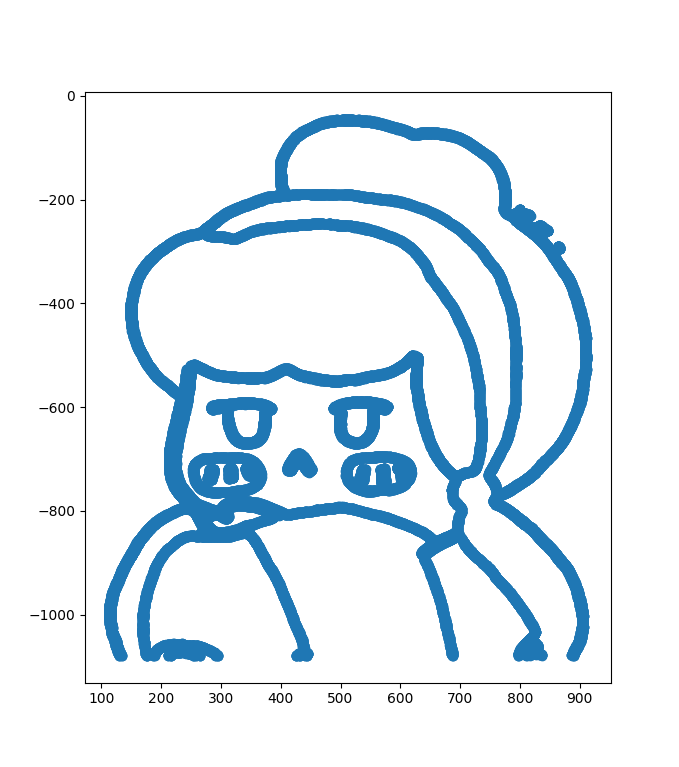
As I am a rookie, I don't know how to display sub-pixel in the image (I hope some big guys can teach me).. Just use a scatter picture. As follows:

Original drawing:

The sub-pixel scatter diagram is:

 

There will be double-layer edges, as follows:

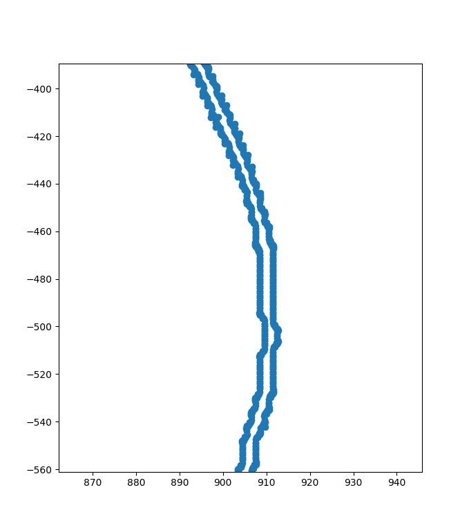
(guess) the reason is that there are pixel differences between the edge line and the background at both ends. If the binary image is detected directly, there should be no double-layer edges.

emmm, the above picture is from the head of your girlfriend.

 

Reference & adapted from: Implementation of sub-pixel edge detection based on Zernike moment_ zilanpotou182 blog - CSDN blog_ opencv sub-pixel edge detection