There are excellent tutorials on the official website of Pytorch. Among them, several short articles belong to the content of the small column called DEEP LEARNING WITH PYTORCH: A 60 MINUTE BLITZ. Considering that it is a little difficult for everyone to read English literature, the author plans to spend some time on translation and make some content adjustments in combination with his own understanding. The original link is posted here Click here to jump . To continue the previous content, click here to jump to Part III . OK, let's start the fourth part and this is the last part.
The content of this part allows us to carry out simple practical combat in combination with our previous knowledge. After learning this part, we can use pytorch to build a simple model, and we will start directly.
Now you know how to define the neural network, calculate the loss value and update the weight value of the neural network. Now I want you to think about it.
What is the data?
Usually, when you have to deal with picture, text, audio and video data, you can use the standard python package to import the data into the numpy array. Then you can convert the array to the tensor type of pytorch.
(1) For pictures, there are pilot and OpenCV packages that can be used.
(2) For audio, packages with scipy and librosa can be used.
(3) For text, both NLTK and SpaCy can be used for loading based on original Python or python
In particular, for visual processing, we have created a package called torchvision, which can be used for data loader of public data sets, such as ImageNet, CIFAR10, MNIST, etc. Data conversion tools for images include torch vision. Datasets and torch.utils.data.DataLoader.
This tool provides us with great convenience, avoids writing too much duplicate code, and is convenient for relevant personnel to use.
For this tutorial, we will use the CIFIA10 dataset. It includes various types, such as' airplane ',' automobile ',' bird ',' cat ',' der ',' dog ',' frog ',' horse ',' ship ',' truck '. These pictures in CIFIA are 3 * 32 * 32 size pictures and 3 (RGB) channel 32 * 32 size pictures.
After the introduction, we will carry out practical training.
Train a picture classifier
We will follow the steps below:
(1) Use torchvision to import and standardize the training data and test data of CIFIA10.
(2) A convolutional neural network is defined
(3) Define a loss function
(4) A neural network is trained on the training data set
(5) Test the effect of the network on the test set
1. Import and normalize the dataset of CIFIA10
Using torchvision, it is very simple to import CIFAR10.
import torch
import torchvision
import torchvision.transforms as transforms
The range of torchvision's dataset output is [0,1]. We convert them into the normalized tensor format, and the range interval is [- 1,1].
transform = transforms.Compose(
    [transforms.ToTensor(),
     transforms.Normalize((0.5, 0.5, 0.5), (0.5, 0.5, 0.5))])

batch_size = 4

trainset = torchvision.datasets.CIFAR10(root='./data', train=True,
                                        download=True, transform=transform)
trainloader = torch.utils.data.DataLoader(trainset, batch_size=batch_size,
                                          shuffle=True, num_workers=2)

testset = torchvision.datasets.CIFAR10(root='./data', train=False,
                                       download=True, transform=transform)
testloader = torch.utils.data.DataLoader(testset, batch_size=batch_size,
                                         shuffle=False, num_workers=2)

classes = ('plane', 'car', 'bird', 'cat',
           'deer', 'dog', 'frog', 'horse', 'ship', 'truck')
If you run on Windows and get a BrokenPipeError, you can Num of torch.utils.data.DataLoader()_ Workers is set to 0.
The output result in the figure above is
Downloading https://www.cs.toronto.edu/~kriz/cifar-10-python.tar.gz to ./data/cifar-10-python.tar.gz
Extracting ./data/cifar-10-python.tar.gz to ./data
Files already downloaded and verified
Since there is no relevant data set on your computer, you will connect to the website for download.
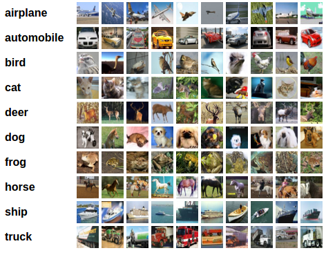
Now let's show the picture of training.
import matplotlib.pyplot as plt
import numpy as np

# functions to show an image


def imshow(img):
    img = img / 2 + 0.5     # unnormalize
    npimg = img.numpy()
    plt.imshow(np.transpose(npimg, (1, 2, 0)))
    plt.show()


# get some random training images
dataiter = iter(trainloader)
images, labels = dataiter.next()

# show images
imshow(torchvision.utils.make_grid(images))
# print labels
print(' '.join('%5s' % classes[labels[j]] for j in range(batch_size)))
The output result is:
cat plane bird ship
2. Define a convolutional neural network
Select a neural network from the neural network set and adjust the input of the network to a 3-channel (RGB) picture instead of the original default single channel (gray) picture.
import torch.nn as nn
import torch.nn.functional as F


class Net(nn.Module):
    def __init__(self):
        super().__init__()
        self.conv1 = nn.Conv2d(3, 6, 5)
        self.pool = nn.MaxPool2d(2, 2)
        self.conv2 = nn.Conv2d(6, 16, 5)
        self.fc1 = nn.Linear(16 * 5 * 5, 120)
        self.fc2 = nn.Linear(120, 84)
        self.fc3 = nn.Linear(84, 10)

    def forward(self, x):
        x = self.pool(F.relu(self.conv1(x)))
        x = self.pool(F.relu(self.conv2(x)))
        x = torch.flatten(x, 1) # flatten all dimensions except batch
        x = F.relu(self.fc1(x))
        x = F.relu(self.fc2(x))
        x = self.fc3(x)
        return x


net = Net()
3. Define a loss function and optimizer
Let's use the loss function of a classifier corss entropy and SGD with momentum.
import torch.optim as optim

criterion = nn.CrossEntropyLoss()
optimizer = optim.SGD(net.parameters(), lr=0.001, momentum=0.9)
4. Training network
The following things begin to become interesting. We simply let the data iterate, feed the input data to the network, and then let the network optimize itself.
for epoch in range(2):  # loop over the dataset multiple times

    running_loss = 0.0
    for i, data in enumerate(trainloader, 0):
        # get the inputs; data is a list of [inputs, labels]
        inputs, labels = data

        # zero the parameter gradients
        optimizer.zero_grad()

        # forward + backward + optimize
        outputs = net(inputs)
        loss = criterion(outputs, labels)
        loss.backward()
        optimizer.step()

        # print statistics
        running_loss += loss.item()
        if i % 2000 == 1999:    # print every 2000 mini-batches
            print('[%d, %5d] loss: %.3f' %
                  (epoch + 1, i + 1, running_loss / 2000))
            running_loss = 0.0

print('Finished Training')
The output result is:
[1,  2000] loss: 2.128
[1,  4000] loss: 1.793
[1,  6000] loss: 1.649
[1,  8000] loss: 1.555
[1, 10000] loss: 1.504
[1, 12000] loss: 1.444
[2,  2000] loss: 1.379
[2,  4000] loss: 1.344
[2,  6000] loss: 1.336
[2,  8000] loss: 1.327
[2, 10000] loss: 1.294
[2, 12000] loss: 1.280
Finished Training
Let's save the model quickly so that we can continue training directly from the parameters here next time.
PATH = './cifar_net.pth'
torch.save(net.state_dict(), PATH)
More details about saving can be viewed Original file.
5. Test the network on the test set
We have trained the network for 2 rounds on the training set (the big cycle of the training network is 2 times), but we need to check whether the network has achieved good learning results.
We detect the error with the real value by detecting the classification of labels and the output of neural network. If the prediction is correct, we will add a sample to the correct prediction set.
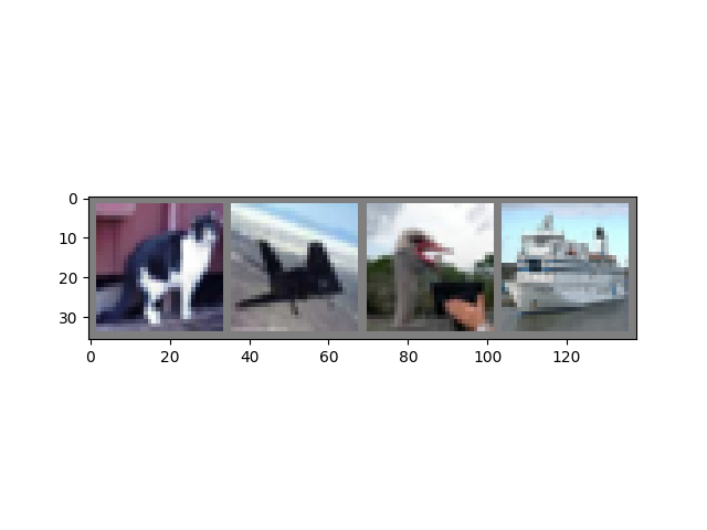
OK, first step, let's show a set of pictures in the self-test set.
dataiter = iter(testloader)
images, labels = dataiter.next()

# print images
imshow(torchvision.utils.make_grid(images))
print('GroundTruth: ', ' '.join('%5s' % classes[labels[j]] for j in range(4)))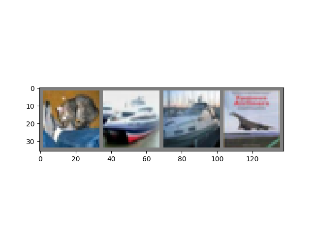
GroundTruth: cat ship ship plane
Next, let's import the model we saved before (in fact, we don't need to save and import the model parameters here. Here's just a demonstration).
net = Net()
net.load_state_dict(torch.load(PATH))
Next, let's think about the above examples of Kangkang neural network:
outputs = net(images)
The output is the probability of 10 categories. The category with the highest probability is identified as the output result, so we will obtain the index of the category with the highest probability.
_, predicted = torch.max(outputs, 1)

print('Predicted: ', ' '.join('%5s' % classes[predicted[j]]
                              for j in range(4)))
The output result is:
Predicted: frog ship ship ship
The results seem good.
Let's see how the network performs on the entire dataset.
correct = 0
total = 0
# since we're not training, we don't need to calculate the gradients for our outputs
with torch.no_grad():
    for data in testloader:
        images, labels = data
        # calculate outputs by running images through the network
        outputs = net(images)
        # the class with the highest energy is what we choose as prediction
        _, predicted = torch.max(outputs.data, 1)
        total += labels.size(0)
        correct += (predicted == labels).sum().item()

print('Accuracy of the network on the 10000 test images: %d %%' % (
    100 * correct / total))
The result output is:
Accuracy of the network on the 10000 test images: 54 %
From the results, it seems that this is much better than taking a chance. Taking a chance is one of ten, that is, the accuracy rate is 10%. It seems that the neural network has something.
Let's see which categories perform better.
# prepare to count predictions for each class
correct_pred = {classname: 0 for classname in classes}
total_pred = {classname: 0 for classname in classes}

# again no gradients needed
with torch.no_grad():
    for data in testloader:
        images, labels = data
        outputs = net(images)
        _, predictions = torch.max(outputs, 1)
        # collect the correct predictions for each class
        for label, prediction in zip(labels, predictions):
            if label == prediction:
                correct_pred[classes[label]] += 1
            total_pred[classes[label]] += 1


# print accuracy for each class
for classname, correct_count in correct_pred.items():
    accuracy = 100 * float(correct_count) / total_pred[classname]
    print("Accuracy for class {:5s} is: {:.1f} %".format(classname,
                                                   accuracy))
The output result is:
Accuracy for class plane is: 59.4 %
Accuracy for class car   is: 66.7 %
Accuracy for class bird  is: 22.7 %
Accuracy for class cat   is: 52.7 %
Accuracy for class deer  is: 59.1 %
Accuracy for class dog   is: 28.9 %
Accuracy for class frog  is: 70.8 %
Accuracy for class horse is: 57.6 %
Accuracy for class ship  is: 67.4 %
Accuracy for class truck is: 62.2 %
OK, what can we do next? We can try GPU acceleration again.
Training on GPU
Just like converting the tensor to the GPU, here we convert the network to the GPU.
If we can get CUDA (NVIDIA's library here for more details, we will continue to write relevant tutorials later), we can first define our device as the first visible CUDA device.
device = torch.device("cuda:0" if torch.cuda.is_available() else "cpu")

# Assuming that we are on a CUDA machine, this should print a CUDA device:

print(device)
The output result is:
cuda:0
The rest assumes that CUDA is already installed on our device.
These methods recursively traverse all modules and convert their parameters and buffers to CUDA's tensor s.
net.to(device)
Remember, you must send the input and target to the GPU at each step Participate in the operation.
inputs, labels = data[0].to(device), data[1].to(device)
If you don't notice more acceleration with the GPU during the test. Mainly because your network may be small.
Try to increase the width of your network and see what kind of acceleration you get.
Through this study, you can establish a small network for image classification. Next, you can further understand PyTorch's library, and then train more neural networks.