The main task of Task 2 is data exploratory analysis

1, EDA introduction and purpose

Introduction:

EDA (exploratory data analysis) refers to a data analysis method that explores the existing data under as few a priori assumptions as possible and explores the structure and law of the data by means of drawing, index, equation fitting, calculation of characteristic quantity and so on. Unlike the initial data analysis, it focuses more on checking the assumptions required for model fitting and hypothesis testing, dealing with missing values, and transforming variables as needed.
Personally, I think this is the first and very important part of data analysis. All subsequent analysis and modeling are based on this step.

Purpose:

1. What is the overall situation of the data?
2. How is the data missing? Is the missing data abandoned or supplemented? What is the way to supplement?
3. What about outliers? How to deal with it?
4. What is the relationship between the variables? What is the relationship between the predicted value and the variables?

2, Code

2.1 guide package and loading data

import warnings
warnings.filterwarnings('ignore')

import pandas as pd
import numpy as np
import matplotlib.pyplot as plt
import seaborn as sns
import missingno as msno

data_train = pd.read_csv('used_car_train_20200313.csv', sep=' ')
data_test_a = pd.read_csv('used_car_testA_20200313.csv', sep=' ')

2.2 viewing basic data information

data_train.sample(10)
data_test_a.head().append(data_test_a.tail())

data_train.shape
data_test_a.shape

data_train.info()
data_test_a.info()

Through the above steps, you can have a preliminary understanding of the data, such as the number of rows and columns, column value type, general structure, data integrity and descriptive statistics of each variable.

2.3 check for missing data

data_train.isnull().sum()
data_test_a.isnull().sum()

Through the missing inspection, it is found that_ A small amount of model, bodyType, fuelType and gearbox are missing in the train, and data is missing_ test_ bodyType, fuelType and gearbox in a, variables with missing values should all have a great impact on the price. Overall, the data integrity is good.

Null value filling method:
Small quantity: the filling of mean value and mode can be considered, or it can be optimized by tree model.
Large quantity: consider deleting.

• Visual analysis

# Null value, visualization, histogram
missing = data_train.isnull().sum()
missing = missing[missing > 0]
missing.plot(kind='bar')

# Using missingno to visualize the missing value library
msno.matrix(data_train)

The more white lines, the more missing values.

# Histogram
msno.bar(data_train)

The lower the column, the more missing values.

Through the missingno library, you can also intuitively see the missing value of the variable.

2.3 check for abnormal data

# View method 1: count the value and number of a column
df['col_name'].value_counts().sort_index()

# Descriptive statistics method: View column 2
df.describe()['col_name']

Through the above methods, you can basically judge the abnormal data. After viewing all columns, you can find that there is an abnormal value '-' in notrepairedamage

data_train['notRepairedDamage'].value_counts()

'-' is also null in nature and can be set to nan

data_train['notRepairedDamage'].replace('-', np.nan, inplace=True)

Then through DF isnull(). The sum () command can view the situation after replacement. The null value of notrepairedamage changes from 0 to 24324 (the number of original '-' values)

Through anomaly detection, it is also found that the category characteristics of seller and offerType fields are seriously inclined, which can be deleted for the help of predicting everything.

# del df['col_name] and DF Drop() is OK

del data_train['seller']
del data_train['offerType']

After deletion, you can use DF Columns.
For data_test_a the same treatment is adopted.

Refer to the following for general ideas and handling methods of data exception inspection:
https://blog.csdn.net/weixin_40444270/article/details/108920646

2.4 distribution of predicted values

2.4.1 simple view

data_train['price']

data_train['price'].value_counts().sort_index()

2.4.2 overall distribution

In machine learning, the research with probability distribution as the core mostly focuses on the normal distribution, which only depends on two characteristics of the data set: the mean and variance of the sample. Using normal distribution, the probability of predicting a variable and finding it within a certain range becomes very simple.
What if the sample does not obey the normal distribution? We can convert it into normal distribution, such as linear transformation, Boxcox transformation and Yeo johnso transformation.
Of course, we can't blindly assume that the variables conform to the normal distribution. For example, it has obvious defects to assume that the stock price follows the normal distribution, because the stock price has no negative number, but we can assume that the stock price serves the lognormal distribution. In addition to normal distribution, variables can also obey Poisson distribution, student t-distribution, binomial distribution and so on.

When the sample data shows that the distribution of quality characteristics is non normal, the application of the method based on normal distribution will make an incorrect decision. Johnson distribution family is the probability distribution of random variables that obey normal distribution after John transformation. Johnson distribution system establishes three families of distributions, which are bounded, lognormal and unbounded.

Next, let's see what the data set conforms to the overall distribution. Unbounded Johnson distribution? Normal distribution? Lognormal distribution?

import scipy.stats as st

y = data_train['price']
plt.figure(1); plt.title('Johnson SU') # Unbounded Johnson distribution
sns.distplot(y, kde=False, fit=st.johnsonsu)

plt.figure(2); plt.title('Normal') # Normal distribution
sns.distplot(y, kde=False, fit=st.norm)

plt.figure(3); plt.title('Log Normal') # Lognormal distribution
sns.distplot(y, kde=False, fit=st.lognorm)

price does not obey the normal distribution and must be converted before regression. It can be seen that it fits better with unbounded Johnson distribution.

2.4.3 viewing Skewness and Kurtosis

• Skewness:
  It is a statistic that describes the distribution form of data. It describes the symmetry of a total value distribution. In short, it is the degree of data asymmetry. The greater the absolute value, the more asymmetric the data distribution and the greater the degree of skewness
  The skewness of normal distribution is 0, that is, the data distribution is symmetrical. If the skewness is > 0, the distribution is to the right, and the long tail of the distribution is to the right. The greater the absolute value of skewness, the more serious the deviation of distribution (Note: left / right deviation refers to the trailing direction of value, not the peak position)
• Kurtosis:
  A statistic that describes the steepness and slowness of the distribution form of all values of a variable. In short, it is the sharpness of the top of the data distribution (> 0 sharp peak, < 0 flat peak, = 0, which is consistent with the steepness of the normal distribution)

print("Skewness: %f" % y.skew())
print("Kurtosis: %f" % y.kurt())

The results show that the price distribution is right and sharp, which is consistent with the figure.
We can also take a look at data_ Skewness and kurtosis of each variable in the train dataset.

sns.distplot(data_train.skew(), color='red', axlabel='Skewness')
sns.distplot(data_train.kurt(), color='blue', axlabel='Kurtosis')

2.4.4 frequency of viewing predicted value

plt.hist(y, orientation='vertical', color='orange') # The parameter orientation determines whether the vertical axis represents the frequency or the horizontal axis represents the frequency
plt.show()

There are very few values greater than 20000. They can be treated as special values or outliers (filled or deleted)

plt.hist(np.log(y), orientation='vertical', color='orange')
plt.show()

The distribution of prices after log transformation is relatively uniform, so log transformation can be used for prediction, which is also a common method in prediction problems.

2.5 characteristic analysis

Features are divided into type features and digital features.
If there is no label encoding data, DF can be used directly select_ Dtypes().

# Digital features
numeric_features = df.select_dtypes(include=[np.number])
numeric_features.columns

# Type properties
categorical_features  = df.select_dtypes(include=[np.object])
categorical_features.columns

However, in this example, there is label encoding, so it needs to be distinguished artificially according to the actual meaning.

numeric_features = ['power', 'kilometer', 'v_0', 'v_1', 'v_2', 'v_3', 'v_4', 'v_5', 'v_6', 'v_7', 'v_8', 'v_9', 'v_10', 'v_11', 'v_12', 'v_13','v_14' ]

categorical_features = ['name', 'model', 'brand', 'bodyType', 'fuelType', 'gearbox', 'notRepairedDamage', 'regionCode']

2.5.1 category feature analysis

1. View feature nunique distribution

for cat_fea in categorical_features:
    print(cat_fea + "The characteristic distribution of is as follows:")
    print("share{}Different values".format(data_train[cat_fea].nunique()))
    print(data_train[cat_fea].value_counts)

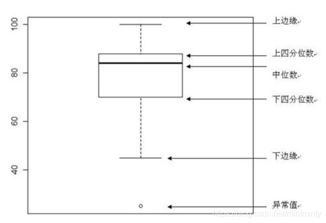
2. Category feature box diagram visualization

• Visually identify outliers in data
• Intuitively judge the discrete distribution of data and understand the data distribution state
  

categorical_features = ['model','brand','bodyType','fuelType','gearbox','notRepairedDamage']

# Convert to classified data
for c in categorical_features:
    data_train[c] = data_train[c].astype('category')
    if data_train[c].isnull().any():
        data_train[c] = data_train[c].cat.add_categories(['MISSING'])
        data_train[c] = data_train[c].fillna('MISSING')
        
# Box diagram, mainly for rotating x-axis coordinates
def boxplot(x, y, **kwargs):
    sns.boxplot(x=x, y=y)
    x = plt.xticks(rotation=90)

f = pd.melt(data_train, id_vars=['price'], value_vars=categorical_features) # price columns that do not need to be converted
g = sns.FacetGrid(f, col='variable', col_wrap=2, sharex=False, sharey=False, size=5)
g = g.map(boxplot, "value", "price")

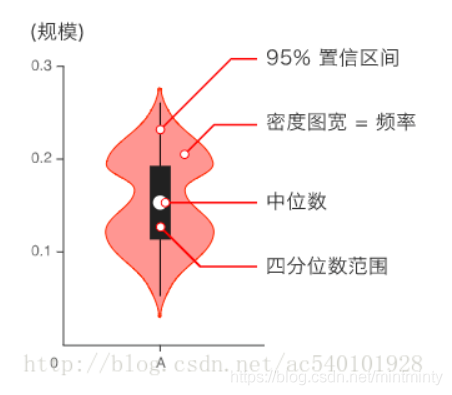
3. Category feature map visualization

• Used to display data distribution and probability density
• This chart combines the characteristics of box chart and density chart, and is mainly used to show the distribution shape of data
  

for c in categorical_features:
    sns.violinplot(x=c, y='price', data=data_train)
    plt.show()

3. Category feature bar chart visualization

for c in categorical_features:
    sns.barplot(data_train[c], data_train['price'])
    plt.xticks(rotation=90)
    plt.show()
    

Black lines are error bars. Error bars are commonly used for statistical or scientific data to show potential errors or uncertainty relative to each data marker in the series. The error line can be used as standard deviation (mean deviation) or standard error.

• 1) Mean ± standard deviation (mean ± SD)
• 2) Mean ± standard error (mean ± SEM)

4. Category characteristics visualization of frequency of each category

def count_plot(x, **kwargs):
    sns.countplot(x=x)
    x = plt.xticks(rotation=90)
    
f = pd.melt(data_train, value_vars=categorical_features)
g = sns.FacetGrid(f, col='variable', col_wrap=2, sharex=False, sharey=False, size=5)
g = g.map(count_plot, "value")

2.5.2 digital feature analysis

Overview

numeric_features.append('price')
data_train[numeric_features].head()

1. Correlation analysis

Before correlation analysis, we need to understand three concepts: dimension, covariance and correlation coefficient. A variable is a dimension. Covariance is defined as E { [ X − E ( X ) ] [ Y − E ( Y ) ] } E\{[X-E(X)][Y-E(Y)]\} The − product of X and Y is usually the difference between X and y. The correlation coefficient is C o v ( X , Y ) / [ σ ( X ) σ ( Y ) ] Cov(X,Y)/[\sigma(X)\sigma(Y)] Cov(X,Y)/[ σ (X) σ (Y) ], recorded as ρ X Y \rho XY ρ XY, where σ ( X ) \sigma(X) σ (10) And σ ( Y ) \sigma(Y) σ (Y) Represents the standard deviation of X and Y respectively, so the correlation coefficient is the product of the covariance of the two variables divided by their standard deviation.
If an observation has p dimensions, calculating the covariance between each dimension and all dimensions will form a p ∗ p p * p p * p matrix. Each number of the matrix is the covariance between its corresponding dimensions. This matrix is called the covariance matrix. The covariance matrix can be further calculated according to the above method to obtain the correlation matrix.

price_numeric = data_train[numeric_features]
price_numeric.corr()

The above code can generate correlation coefficients between all dimensions. Let's take out the price column separately.

price_numeric.corr()['price'].sort_values(ascending=False)

Next, use SNS Heatmap () for visualization, and the thermal map has a strong visualization effect on the correlation coefficient of the data set.

correlation = price_numeric.corr()
f, ax = plt.subplots(figsize=(7,7))
plt.title('Correlation of Numeric Features with Price',y=1,size=16)
sns.heatmap(correlation)

sns.heatmap() common optional parameters:

• annot: the default is False. When True, numbers will be displayed on the grid
• vmax, vmin: the maximum and minimum values of the color values of the thermal diagram, which will be exported from data by default.
• Square: whether it is a square. The default value is True.

2. View characteristic skewness and kurtosis

for col in numeric_features:
    print('{:15}'.format(col), 
         'Skewness: {:5.2f}'.format(data_train[col].skew()), #{: 05.2f} 5-digit width, 2-digit decimals
         '    ',
          'Kurtosis: {:06.2f}'.format(data_train[col].kurt())  
         )

3. Visualization of the distribution of each digital feature

• pd.melt(): in data analysis, it is often necessary to convert wide data into long data, similar to column to row.
• sns.FacetGrid(): draw multiple variables without writing a loop. FacetGrid is a class in seaborn library. When initializing this class, we only need to pass it a DataFrame dataset (long data is accepted). After instantiating this class, you can directly use the method of this object to draw the required graphics. map can be self-defined functions, SNS, plt, etc.

f = pd.melt(data_train, value_vars=numeric_features)
g = sns.FacetGrid(f, col="variable",  col_wrap=2, sharex=False, sharey=False)
g = g.map(sns.distplot, "value")

According to the results, we can see that the distribution of anonymous features is relatively uniform.

4. Visualization of the relationship between digital features

• sns.pairplot(): it can also be seen from pair that this shows the relationship between two. On the diagonal line is the histogram (distribution map) of each attribute, which can be obtained through the parameter diag_kind setting, rather than diagonal, is the correlation graph between two different attributes.

# Here is to select the top 10 ones with high correlation with price for visualization
columns = ['price', 'v_12', 'v_8' , 'v_0', 'power', 'v_5',  'v_2', 'v_6', 'v_1', 'v_14']
sns.pairplot(data_train[columns], size = 2 ,kind ='scatter',diag_kind='kde')
plt.show()

As we can see from the figure, v_6 and V_ There is an obvious relative relationship between them.

5. Regression relationship between multivariate and price

• sns.regplot(): plot data and linear regression model fitting

2.6 using pandas_ Generating data report

pandas_profiling, this library only needs one line of code to generate data EDA reports.

import pandas_profiling

pfr = pandas_profiling.ProfileReport(data_train)
pfr.to_file('example.html')

3, Summary

This part took me a lot of time and learned a lot. I also reviewed a lot of basic knowledge about distribution and the Johnson distribution I heard for the first time... The foundation is too weak. I have to learn how pairplot looks at relevance. Many of them can't be found on Baidu. I asked a lot of teaching assistants of datawahle. In short, I have learned a lot through stumbling. I still need to continue my efforts. I am still very happy with the harvest. Thank you very much for your help!!
The knowledge of statistics must be well studied, well studied!! It is the soul of data analysis.