Research on background noise

1. How is sound generated?
Sound is a wave phenomenon that is generated by the vibration of an object, propagates through a medium (air or solid, liquid) and can be perceived by human auditory organs.
An object that initially vibrates. Sound vibrates and propagates in the form of waves, so sound is a kind of wave.
2. The significance of signal processing?
The essence of sound is pressure pulsation, so whether it is simulation or experiment, what is directly measured is only the pressure value at each time. Although we can qualitatively judge the strength of the pressure pulsation by the size of the pressure signal in the time domain, the time signal of the pressure is too chaotic. We usually need to convert the time domain signal into the frequency domain in order to more clearly identify the characteristics of the signal.
3. Time domain and frequency domain?
Time domain: the coordinate system that describes the change of signal with time.
Frequency domain: a coordinate system used to describe the frequency characteristics of signals. Its abscissa is the frequency.
For an object with a specific geometric scale, the number of times the air flow sweeps it in one second is the frequency, so the faster the speed, the higher the signal frequency; The frequency is often inversely proportional to the geometric scale, that is, the smaller the size, the higher the frequency. Compared with the time domain, the signal in frequency domain is easier to establish a corresponding relationship with the geometric structure and flow field.
4. How to convert?
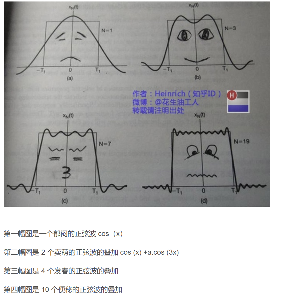
Fourier principle: any continuously measured time-domain signal can be expressed as the infinite superposition of sine wave signals of different frequencies. Fourier transform is an integral transform method to recover and convert these sine wave signals into frequency domain space.

For discrete-time serial number signals x ( j ) , j = 1 , 2 , 3 , ... , N x(j),j=1, 2, 3, \dots, N x(j),j=1,2,3,..., N, its Fourier transform and its inverse transform can be expressed as:
Y ( K ) = ∑ j = 1 N x ( j ) W N ( j − 1 ) ( k − 1 ) Y(K) = \sum_{j=1}^{N}x(j)W_N^{(j-1)(k-1)} Y(K)=j=1∑N​x(j)WN(j−1)(k−1)​
x ( j ) = 1 n ∑ k = 1 N Y ( k ) W N − ( j − 1 ) ( k − 1 ) x(j) = \frac{1}{n}\sum_{k=1}^NY(k)W_N^{-(j-1)(k-1)} x(j)=n1​k=1∑N​Y(k)WN−(j−1)(k−1)​
Among them, W N = e ( − 2 π i ) / N W_N=e^{(-2\pi i)/N} WN​=e(−2πi)/N.
Discrete Fourier transform is also a transformation from time domain to frequency domain, but it is a set of complex numbers x ( j ) x(j) x(j), converted to another set of complex numbers Y ( K ) Y(K) Y(K), you can happily realize the transformation of discrete data.
Discrete Fourier transform is good, but if the amount of sampled data is large, the amount of calculation will increase sharply. In 1965, Cooley and Tukey proposed a fast algorithm for discrete Fourier transform (DFT), namely fast Fourier transform.
5. Spectrum
We know that the abscissa of the spectrum is the frequency, and the ordinate represents the amplitude at this frequency, which is the strength of the pressure pulsation for the sound signal.
6. Realize Fourier transform in matlab

Ts = 1/50;
t = 0:Ts:10-Ts;
x = sin(2*pi*15*t) + sin(2*pi*20*t);
plot(t,x)% Abscissa is time and ordinate is value
xlabel('Time(seconds)')
ylabel('Amplitude')
y = fft(x);
fs = 1/Ts;
f = (0:length(y)-1)*fs/length(y);%Set Fourier transform y Is the longitudinal axis, f Is the horizontal axis
plot(f,abs(y))%Finally, the frequency domain diagram is generated
xlabel('Frequency(Hz)')
ylabel('Magnitude')
title('Magnitude')
%fftshift Function performs a zero centered circular translation on the transform
n = length(x);
fshift = (-n/2:n/2-1)*(fs/n);
yshift = fftshift(y);
plot(fshift,abs(yshift))
xlabel('Frequency (Hz)')
ylabel('Magnitude')
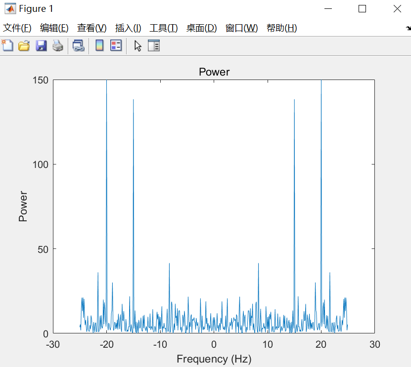
rng('default')
xnoise = x + 2.5*randn(size(t));%stay x Gaussian noise mixed in
%Painting noisy images
ynoise = fft(xnoise);
ynoiseshift = fftshift(ynoise);
power = abs(ynoiseshift).^2/n;
plot(fshift,power)
title('Power')
xlabel('Frequency (Hz)')
ylabel('Power')
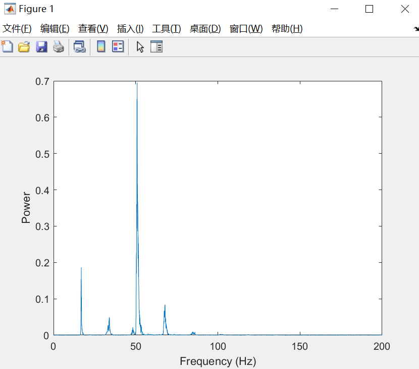
%Computational fast Fourier transform
whaleFile = 'bluewhale.au';
[x,fs] = audioread(whaleFile);
whaleMoan = x(2.45e4:3.10e4);
t = 10*(0:1/fs:(length(whaleMoan)-1)/fs);

plot(t,whaleMoan)
xlabel('Time (seconds)')
ylabel('Amplitude')
xlim([0 t(end)])
m = length(whaleMoan); 
n = pow2(nextpow2(m));
y = fft(whaleMoan,n); 
f = (0:n-1)*(fs/n)/10; % frequency vector
power = abs(y).^2/n;   % power spectrum      
plot(f(1:floor(n/2)),power(1:floor(n/2)))
xlabel('Frequency (Hz)')
ylabel('Power')