1. Introduction to Cellular Automata
Development of 1-cell automata
The original cellular automata was proposed by Von Neumann in the 1950s to mimic the self-replication of biological cells.But it has not been taken seriously by the academia.
It was only after John Horton Conway of the University of Cambridge designed a computer game called "Game of Life" in 1970 that cellular automata caught the attention of scientists.
S.Wolfram published a series of papers in 1983.The model produced by 256 rules of elementary cellular machine is studied in detail, and its evolution behavior is described by entropy. Cellular automata are classified into stationary, periodic, chaotic and complex types.
2 Preliminary Understanding of Cellular Automata
Cellular automata (CA) is a method used to simulate local rules and local connections. A typical CA is defined on a grid, where a grid at each point represents a cell and a limited state. Change rules apply to each cell and occur simultaneously. Typical change rules are determined by the state of the cell and its (4 or 8)Status of the neighbor.
Rule of change of 3-cell-cell state
Typical rules of change depend on the state of the cell and its (4 or 8) neighbors.
Application of 4-cell automata
Cellular automata has been used in physical simulation, biological simulation and other fields.
matlab programming of 5-cell automata
Combining the above, we can understand that cellular automata simulation needs to understand three points. One is a cell, which can be understood in matlab as a square block composed of one or more points in a matrix. Generally, we use one point in the matrix to represent a cell. The second is the change rule, which determines the state of the cell at the next moment. The third is the state of the cell, which is customized.Is usually an opposite state, such as the living or death state of an organism, a red or green light, the point with or without obstacles, etc.
6-D Cellular Automata-Traffic Rules
Definition:
6.1 cells are distributed on a one-dimensional linear grid.
6.2 cells have only two states, vehicle and empty.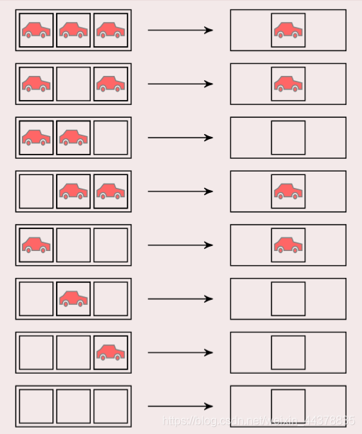
7 2-D Cellular Automata-Game of Life
Definition:
7.1 cells are distributed on a two-dimensional square grid.
7.2 cells have only two states of life and death.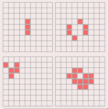
Cell status is determined by the surrounding eight neighbors.
Rules: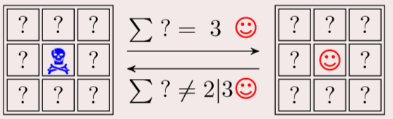
Skull: Death; Smile: Survival
There are three smiling faces around, but they change to smiling faces in the middle
Less than two smiles or more than three, with death in the middle.
8 What is cellular automata
Discrete systems: Cells are defined in limited time and space, and the state of the cell is limited.
Dynamics System: The behavior of cellular automata is characterized by dynamics.
Simple and Complex: Cellular automata simulates complex worlds with cells that control interactions using simple rules.
9 Components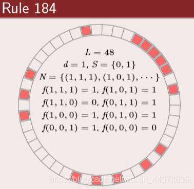
(1) Cells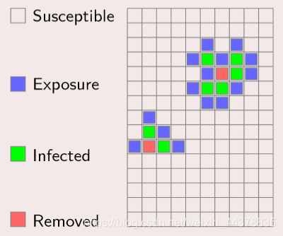
Cells are the basic units of cellular automata:
State: Each cell has the function of remembering the stored state.
Discrete: In simple cases, a cell has only two possible states;In more complex cases, cells have multiple states.
Update: Cell status is constantly updated according to the dynamic rules.
(2) Grid (Lattice)
Different Dimensional Grids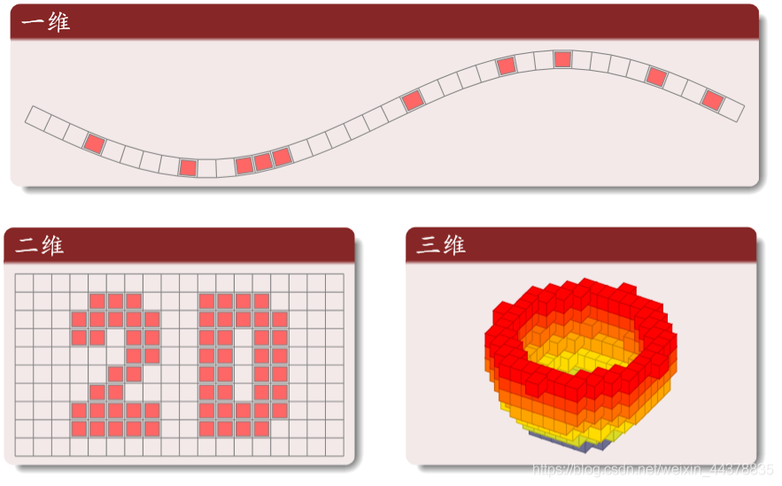
Common 2-D grids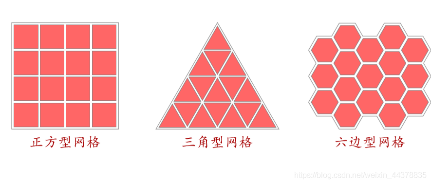
(3) Neighborhood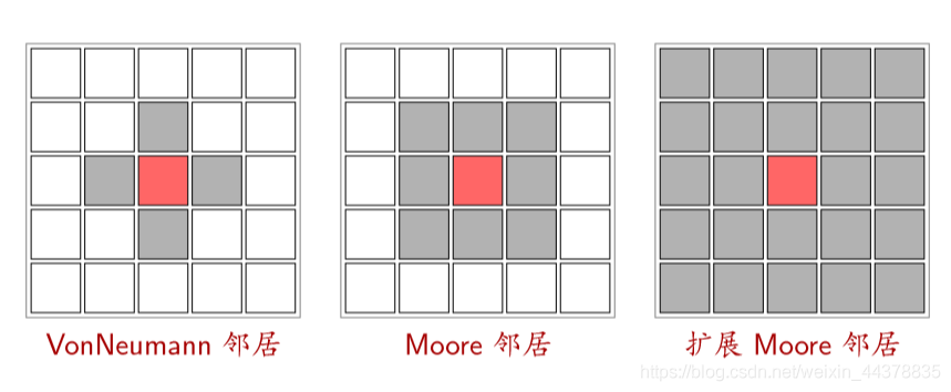
(4) Boundary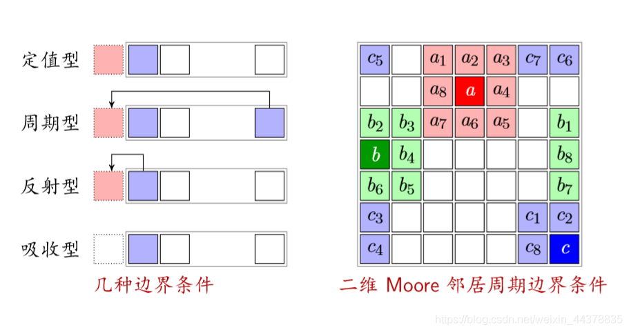
Reflective: A state bounded by itself
Absorption type: regardless of the boundary (the car disappears when it reaches the boundary)
(5) Rules (State Transition Function)
Definition: A dynamic function that determines the state of a cell at the next moment based on its current state and its neighbor state, or simply a state transfer function.
Classification:
Sum type: The state of a cell at the next moment depends on, and only depends on, the current state of all its neighbors and of itself.
Legality type: The summation type rule belongs to the legality type rule.However, if the rules of cellular automata are restricted to the sum type, cellular automata will have limitations.
(6) Forest fires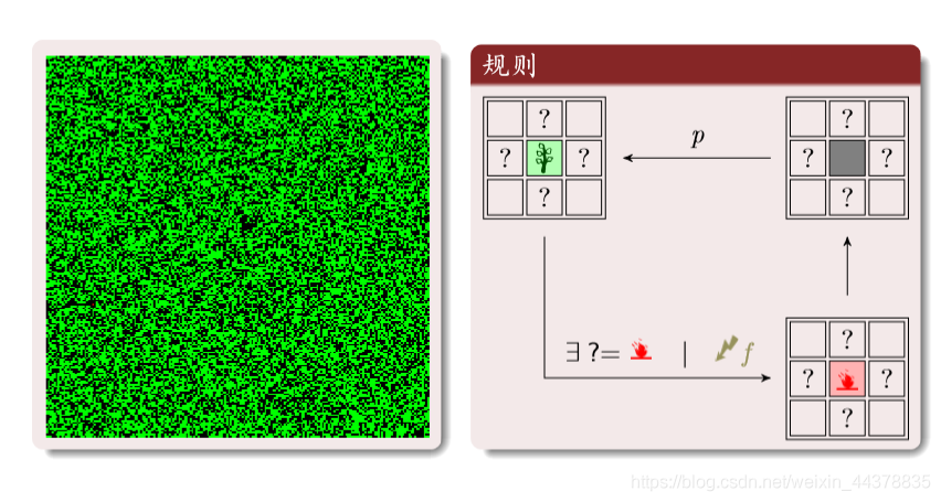
Green: trees; red: fire; black: open space.
Three states cyclic transition:
Tree: Fire turns into fire when there is fire around or when lightning strikes it.
Open space: change to trees with probability p
Rational Analysis: Red is fire; Gray is open space; Green is tree
The density of three states of a cell is 1
The density of fire converted to open space is equal to the density of open space converted to tree (newly grown trees are equal to burned trees)
f is the probability of lightning: much less than the probability of tree generation; T s m a x T_{s m a x}T s m a x
Is the time scale at which a large group of trees was burned
Program implementation
Periodic boundary conditions
Buy it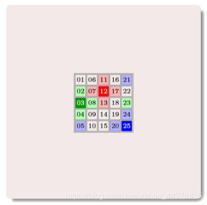
Numbering is the number
Building Neighbor Matrix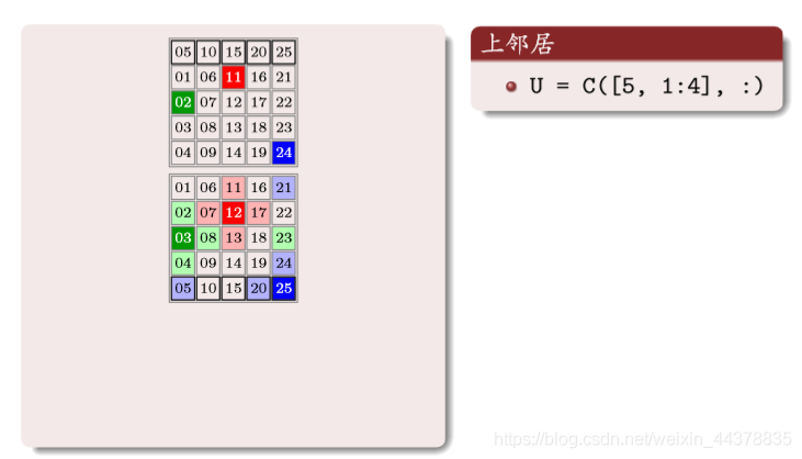
The number in the matrix above corresponds to the upper neighbor number of the same position number of the original matrix, one to one
The same applies: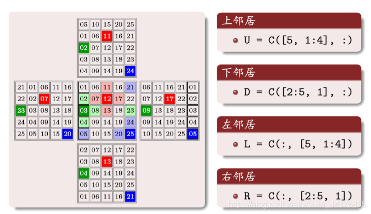
(7) Transportation concepts
Distance and density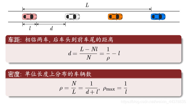
Flow equation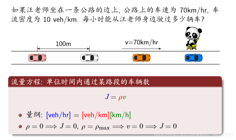
conservation equation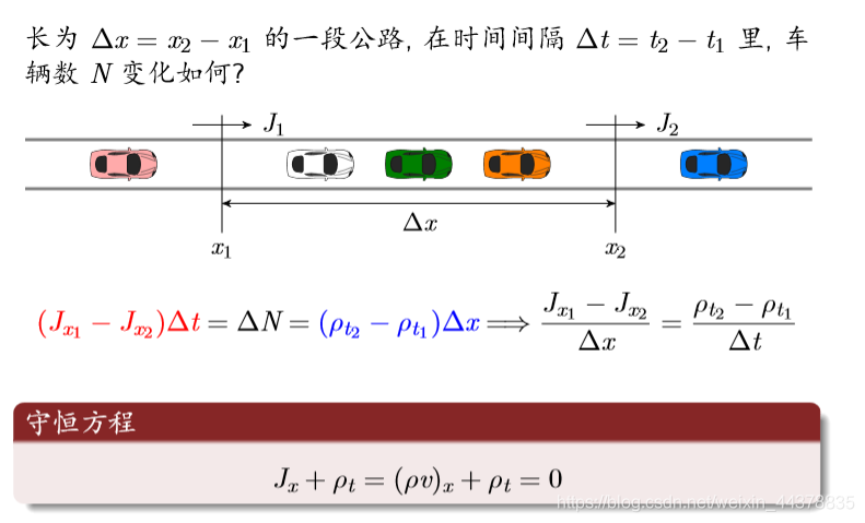
Space-time trajectory (horizontal axis is space vertical axis is time)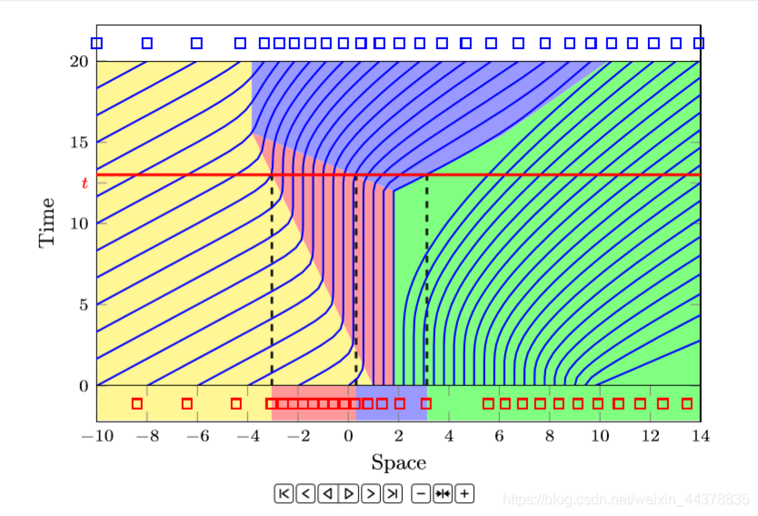
The intersection of the red line and the blue line indicates the location of the car at each time.
Vertical lines indicate the time the car is in that position
Macro Continuous Model: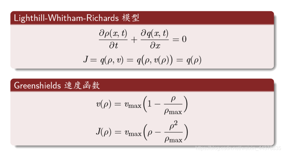
Most commonly used rules: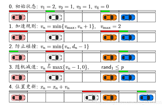
A red bar indicates full speed.
1 Acceleration rule: cannot exceed v m a x (2 lattices / s) v_{m a x} (2 lattices / s) V
max (2 lattices/s)
2 Collision prevention: no more than car distance
Theoretical Analysis: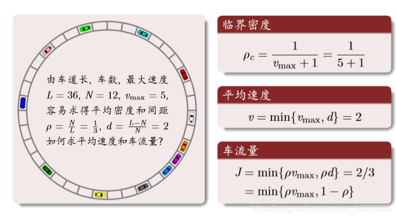
Result analysis: density and flow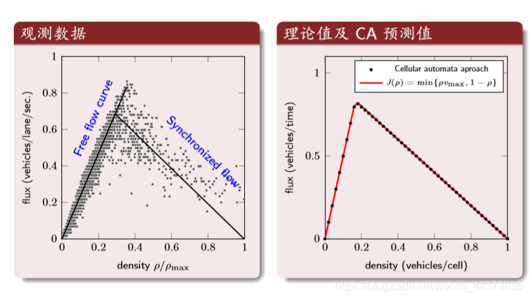
First, the horizontal coordinate is the normalized density and the vertical coordinate is the traffic volume. Second, the theoretical values and the results of CA
Result analysis: space-time trajectories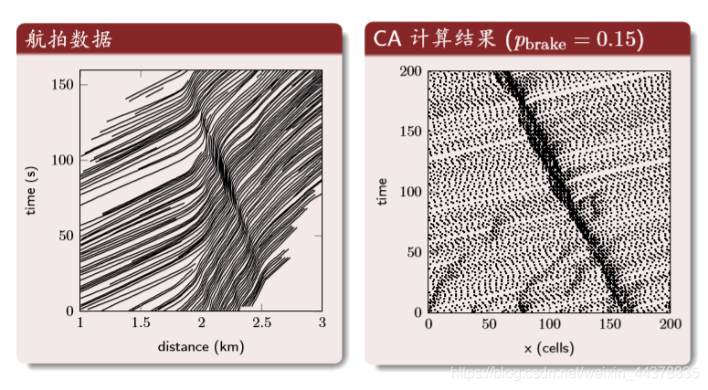
The dark area in the middle is the area with traffic jams.
2. Partial Source Code
function main
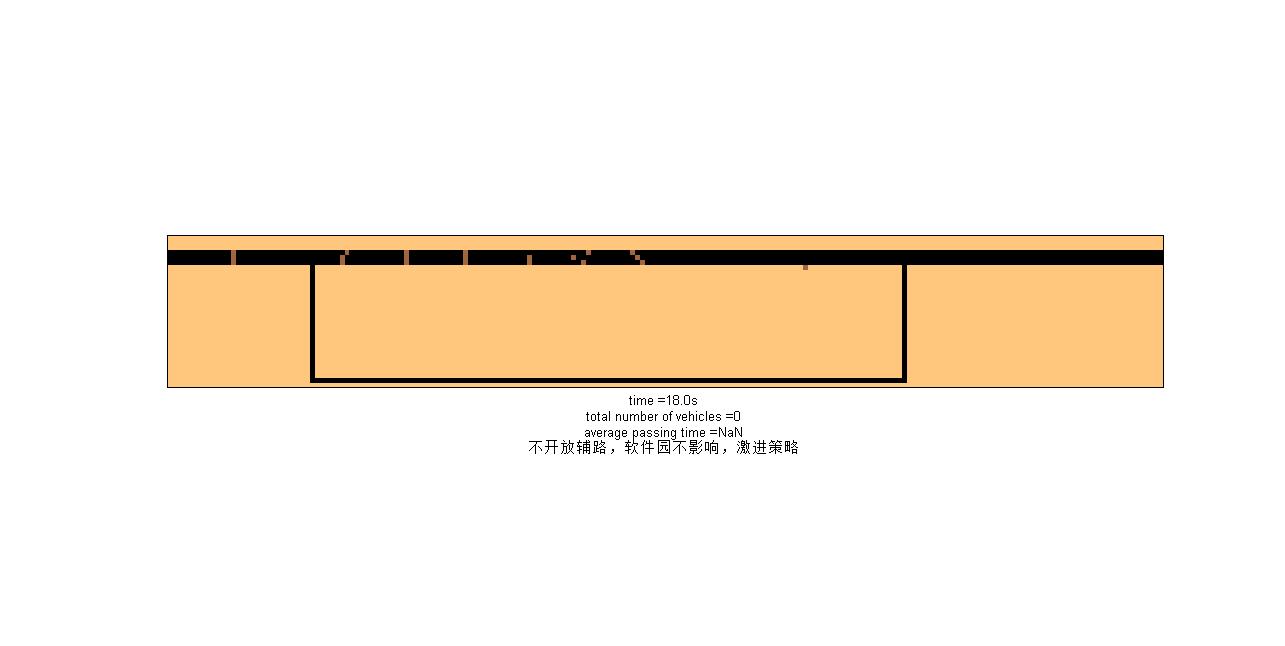
% Cellular Automata Simulation of Peak Hours of Secondary Roads with One Drive on Both Sides of Large Enterprises in the Middle of a Three-lane Trunk Road
% %%%%%%%%%%%%%%%%%%%%%%%%%%%%%%%%%%%%%%%%%%
% Sidex1 Sidex2
% +---------------+ Sidey = 2
% | |
% | |
% ======+===============+==== Mainy
% %%%%%%%%%%%%%%%%%%%%%%%%%%%%%%%%%%%%%%%%
% T Total simulated real time
% Arrival Total Traffic Flow
% Mainlength Trunk road length
% Mainy Avenue ordinates
% Mainwide Main road width
% Sidewide Secondary road width
% Sidex1 Sidex2 Auxiliary road x-coordinates
% Sidey Auxiliary road ordinates
% Sidelengthh Secondary road north-south length
% Sidelengthw Auxiliary road East-West long
% MP map matrix
% 1 Empty 2 Car 3 Boundary
% lightmp Traffic lights
% lighttime Traffic light interval
% v Vehicle Speed Matrix
% vmainmax Highest speed on main road
% vsidemax Auxiliary Highest Speed
% time Car Time Matrix
% dt unit time
% tt Image refresh time
% h handle
% sumtime Total car time
% alltime Total Car Time
% changepro Right Lane Entry Paving Probability
clear;clc
T = 3000;
Mainlength = 200; Mainwide = 3; vmainmax = 6;
%Sidelengthh = 25; Sidelengthw = 100; Sidewide = 1;
vsidemax = 4;
Sidex1 = 30; Sidex2 = 150; Sidey = 2; Mainy = 26;
[mp, v, time,lightmp] = init_mp(Sidex1,Sidex2,Sidey,Mainy,Mainlength,Mainwide);
h = print_mp(mp, NaN, 0.1);
dt = 1.2; tt=0.1;
sumtime = 0; sumpassed =0;
lighttime = 20;
changepro = 0;
alltime=0;
%mp(25,comy)=2;
cy2=130;
mp(25,cy2)=2;
for i = 1:T
sumtime=sumtime+dt;
% Brush Car
if(rem(i,2)&(mp(27,8)~=2||v(27,8)~=0))[mp, v] = new_cars(dt,mp,v,vmainmax); end;
% Software Park
% if(rem(i,2))mp(24,cy2)=1;else mp(24,cy2)=2;end;
% mp(26,cy2)=2;v(26,cy2)=0;
% Variation chos_road2 radical chos_road Conservative
[mp, v, time] = chos_road(mp,v,time);
% variable speed
[mp, v, time] = change_speed(mp,v,time,vmainmax);
flag = (mp(Mainy,Sidex2)==0)
% Accessory Road
if(flag)
[mp, v, time] = fulu(mp,v,time,vsidemax,Sidex1,Sidex2,Sidey,changepro);
end;
% displacement&Car stop
[alltime, mp, v, time , sumpassed ] = move(alltime,sumpassed,mp,v,time,dt);
% Accessory Road
if(~flag)
[mp, v, time] = fulu(mp,v,time,vsidemax,Sidex1,Sidex2,Sidey,changepro);
end;
function [mp, v, time] = chos_road(mp,v,time)
%
%
%
%
%
%
%
[N, M] = size(mp);
for y=M-1:-1:2
for x=26:28
if(mp(x,y)==2 & mp(x,y+1)~=1)
if(mp(x-1,y)==1 & mp(x+1,y)==1 )
if(rand<0.5)
mp(x+1,y)=2;
mp(x,y)=1;
v(x+1,y)=v(x,y);
v(x,y)=0;
time(x+1,y)=time(x,y);
time(x,y)=0;
else
mp(x-1,y)=2;
mp(x,y)=1;
v(x-1,y)=v(x,y);
v(x,y)=0;
time(x-1,y)=time(x,y);
time(x,y)=0;
end;
elseif(mp(x+1,y)==1)
mp(x+1,y)=2;
mp(x,y)=1;
v(x+1,y)=v(x,y);
v(x,y)=0;
time(x+1,y)=time(x,y);
time(x,y)=0;
elseif(mp(x-1,y)==1)
mp(x-1,y)=2;
mp(x,y)=1;
v(x-1,y)=v(x,y);
v(x,y)=0;
time(x-1,y)=time(x,y);
time(x,y)=0;
end;
end;
end;
end;
function [mp, v, time] = chos_road(mp,v,time)
%
%
%
%
%
%
%
[N, M] = size(mp);
dis=zeros(N,M)-1;
for y=M:-1:2
for x=26:28
if (mp(x,y)==2|mp(x,y)==3)
dis(x,y) = 0;
end;
end;
end;
for y=M-1:-1:2
for x=26:28
if (dis(x,y)==-1 && dis(x,y+1)~=-1 )
dis(x,y) = dis(x,y+1)+1;
end;
end;
end;
for y=2:M-1
for x=26:28
if(mp(x,y)==2)
if(dis(x,y+1)==-1)dis(x,y)=123;
else dis(x,y)=dis(x,y+1)+1;
end;
end;
end;
end;
for y=2:M-1
for x=26:28
if(mp(x,y)==2 & (dis(x,y)-1<v(x,y)||mp(x,y+1)==2))
if(mp(x-1,y)==1 & dis(x-1,y)>dis(x,y) & mp(x+1,y)==1 & dis(x+1,y)>=dis(x,y))
if(rand<0.5)
mp(x+1,y)=2;
mp(x,y)=1;
v(x+1,y)=v(x,y);
v(x,y)=0;
time(x+1,y)=time(x,y);
time(x,y)=0;
else
mp(x-1,y)=2;
mp(x,y)=1;
v(x-1,y)=v(x,y);
v(x,y)=0;
time(x-1,y)=time(x,y);
time(x,y)=0;
end;
elseif(mp(x+1,y)==1 & dis(x+1,y)>=dis(x,y))
mp(x+1,y)=2;
mp(x,y)=1;
v(x+1,y)=v(x,y);
v(x,y)=0;
time(x+1,y)=time(x,y);
time(x,y)=0;
elseif(mp(x-1,y)==1 & dis(x-1,y)>dis(x,y))
mp(x-1,y)=2;
mp(x,y)=1;
v(x-1,y)=v(x,y);
v(x,y)=0;
time(x-1,y)=time(x,y);
time(x,y)=0;
end;
end;
end;
end;
3. Operation results
4. matlab Versions and References
1 matlab version
2014a
2 References
[1] Cai Limei. MATLAB Image Processing - Theory, Algorithm and Example Analysis [M]. Tsinghua University Press, 2020.
[2] Yang Dan, Zhao Haibin, Longzhe.MATLAB image processing example in detail [M]. Tsinghua University Press, 2013.
[3] Zhou Pin. MATLAB Image Processing and Graphical User Interface Design [M]. Tsinghua University Press, 2013.
[4] Liu Chenglong. Proficient in MATLAB image processing [M]. Tsinghua University Press, 2015.
[5] Meng Yifan, Liu Yijun. Research on face recognition method based on PCA-SVM [J]. Science and technology horizon.2021, (07)
[6] Zhang Na, Liu Kun, Han Meilin, Chen Chen Chen. A face recognition algorithm based on PCA and LDA fusion [J]. Electronic measurement technology.2020,43(13)
[7] Chen Yan. Analysis of face recognition method based on BP network [J]. Information and computer (theoretical version).2020,32 (23)
[8] Dai Lirong, Chen Wanmi, Guo Sheng. Face recognition research based on skin color model and SURF algorithm [J]. Industrial control computer.2014,27 (02)