1. WSN Model

1.1 Motivation

In recent years, with the development of distributed environment such as peer-to-peer network, cloud computing and grid computing, wireless sensor network (WSN) has been widely used.Is a new computing and network mode that can be defined as a network of tiny, small, expensive and highly intelligent devices called sensor nodes. Sensor nodes are located in different locations in the observed space and exchange data collected from the monitoring area through wireless communication channels. The collected data is sent to the sink node, which is either local or local.Processing data, or sending data to other networks with greater processing power.

One of the most basic challenges in wireless sensor networks is node positioning. There are many examples of node positioning problems, which are NP-hard optimization problems. Traditional deterministic techniques and algorithms cannot solve NP-hard problems within a reasonable computing time. In this case, it is better to use non-deterministic (random) algorithms, such as meta-heuristic algorithms.

Group Intelligence Metaheuristic algorithms simulate biological groups in nature, such as those of birds and fish, bees and ants, bats and azaleas. These algorithms are population-based, random and iterative search methods based on four self-organizing principles: positive feedback, negative feedback, multiple interactions and fluctuations.

1.2 Location issues in Wireless Sensor Networks

Location is one of the most studied problems in wireless sensor networks because coverage, power and routing cannot be optimized if the location of sensor nodes is unknown. Location is the key to wireless sensor networks. The location of some sensor nodes can be determined by Global Positioning System (GPS).To define, these nodes are called anchor nodes or beacon nodes, while other sensor nodes are randomly distributed in the search space. These nodes are called unknown nodes or sensor nodes. Because of the factors such as battery life, cost, climate conditions of each node, only a few nodes'positions are determined by GPS coordinates, while the locations of other nodes need to be improved by localization algorithm.Line estimate.

For positioning of sensor nodes in wireless sensor networks, two positioning algorithms, anchor node and unknown node, are proposed. The first phase is called ranging phase, and the algorithm determines the distance between unknown nodes and adjacent anchor nodes. For positioning of sensor nodes in wireless sensor networks, two positioning algorithms, anchor node and unknown node, are proposed. The first phase is called detection.In the second phase, the algorithm determines the distance between unknown nodes and adjacent anchor nodes. In the second phase, the location of nodes is estimated by collecting ranging information using various methods in the first phase, such as angle of arrival (AOA), time of arrival (TOA), time of arrival (TDOA), round-trip time (RTT), wireless signal strength (RSS).

1.3 Question Statement

In a wireless sensor network consisting of M sensor nodes, the target of the positioning problem is to estimate the position of N unknown nodes within the transmission range of R using the location information of M-N anchor nodes. If a sensor node is within the transmission range of three or more anchor nodes, it is considered to be positioned. This is a two-dimensional positioning problem with a total coordinate number of 2n.

This paper uses the RSS method to estimate the distance between nodes. An imprecise measurement may occur regardless of the ranging method used. Location estimation of N unknown node coordinates can be expressed as an optimization problem involving the minimization of the objective function that represents the positioning error of nodes [19]. The objective function of this problem is expressed by the squares of errors between N unknown nodes and M N adjacent anchor nodes.[19].

With the advent of RSS, trilateral measurement will be used to solve the positioning problem in WSN. The principle of this method is based on the known positions of three anchor nodes. The positions of unknown nodes can be estimated within the transmission range of three anchor nodes.

Each node is estimated to have a distance of d_=d i+ni to the first anchor point, where Ni is a Gaussian noise and D I is the actual distance calculated using the following equation:

The objective function that should be minimized is expressed as the mean square error (MSE) between calculating the actual and estimated distances of the node coordinates and the actual node coordinates:

Where d I is the actual distance, d_i is the estimated distance (the value d I measured from the noise range), M is greater than or equal to 3 (the location of the sensor node requires at least three anchors within the transmission range R).

Since distance measurement in node positioning is noisy, optimization methods such as swarm intelligence metaheuristics are used to estimate sufficient distance between nodes.

2. Sparrow algorithm

Optimization is a hot issue in scientific research and engineering practice. Intelligent optimization algorithms are mostly inspired by human intelligence, the social nature of biological groups or the laws of natural phenomena to optimize globally in the solution space. Sparrow algorithm was first proposed by Xue Jiankai [1] in 2020, and it is a new intelligent optimization algorithm based on the foraging and anti-feeding behavior of sparrow population.

Description of the Sparrow Search algorithm and its formula:

Build a sparrow population: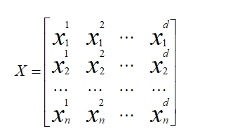

Where d is the dimension of the problem to be optimized and n is the number of sparrows. The fitness function for all sparrows can be expressed as follows:

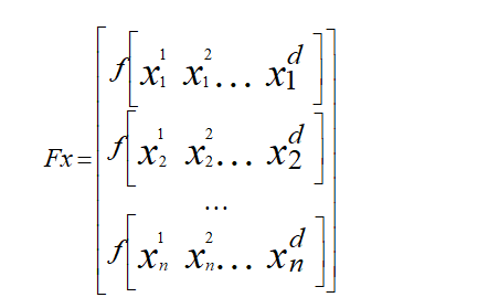
Where Fx represents the fitness function value.

There are two types of sparrows in the sparrow algorithm: discoverer and joiner, who are responsible for finding food for the whole population and providing the direction of feeding for the joiners. Therefore, the search range of the finder is larger than that of the joiners. During each iteration, the finder iterates according to formula (3).

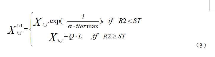
Where t denotes the current iteration number and Xij denotes the location information of the ith sparrow population in the jth dimension.Alpha is a random number from 0 to 1, itermax is a maximum number of iterations, Q is a random number that follows a normal distribution, L is a 1*d matrix with all elements 1, R2 is a 0-1 warning value for sparrow population location, ST is a 0.5-1 warning value for sparrow population location.

When R2<ST indicates that the warning value is less than the safe value, there are no predators in the feeding environment and the discoverer can search extensively. When R2>ST means that some sparrows in the population have already found predators and alerted other sparrows in the population, all of them need to fly to the safe area to feed.

During the feeding process, some participants will always monitor the discoverer. When the discoverer finds better food, the participant will compete with it. If successful, the food of the discoverer will be obtained immediately. Otherwise, the participant will update the location according to formula (4).

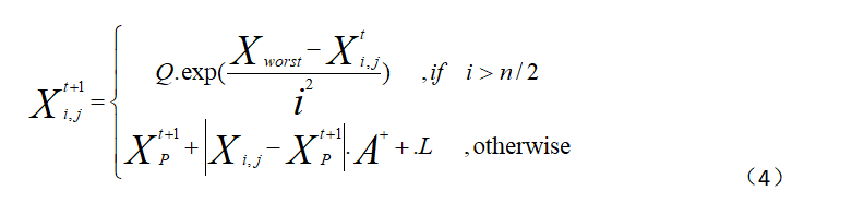
Where XP represents the optimal location discovered by current discoverers, Xword represents the current global worst location, A represents a matrix whose elements are randomly assigned 1*d or -1 and satisfies a relationship:

L is still a 1*d matrix with all elements 1. When i>n/2 this indicates that the first participant is not getting food, is hungry, and needs to fly elsewhere to get more energy.

The number of sparrows in the sparrow population that are aware of danger accounts for 10% to 20% of the total population. The location of these sparrows is randomly generated and updated according to formula (5).

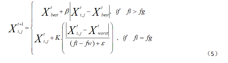
Here, Xbest indicates the current global optimal position, is a random number obeying the standard normal distribution used as the step control parameter, Beta is a random number belonging to -1 to 1, FI is the current fitness value of sparrow individuals, FG is the global optimal fitness value, fw is the global worst fitness value, like the left ear is this read "no laundering"? "No laundering"Represents a constant that avoids zero denominator. When fi > fg, the sparrow is at the edge of the population and vulnerable to predators. When fi=fg, the sparrow in the middle of the population is also at risk and needs to be close to other sparrows to reduce the risk of being preyed.

3. Code

function [FoodFitness,FoodPosition,Convergence_curve]=SSA(N,Max_iter,lb,ub,dim,fobj)
if size(ub,1)==1
    ub=ones(dim,1)*ub;
    lb=ones(dim,1)*lb;
end
Convergence_curve = zeros(1,Max_iter);
%Initialize the positions of salps
SalpPositions=initialization(N,dim,ub,lb);
FoodPosition=zeros(1,dim);
FoodFitness=inf;
%calculate the fitness of initial salps
for i=1:size(SalpPositions,1)
    SalpFitness(1,i)=fobj(SalpPositions(i,:));
end
[sorted_salps_fitness,sorted_indexes]=sort(SalpFitness);
for newindex=1:N
    Sorted_salps(newindex,:)=SalpPositions(sorted_indexes(newindex),:);
end
FoodPosition=Sorted_salps(1,:);
FoodFitness=sorted_salps_fitness(1);
%Main loop
l=2; % start from the second iteration since the first iteration was dedicated to calculating the fitness of salps
while l<Max_iter+1
    c1 = 2*exp(-(4*l/Max_iter)^2); % Eq. (3.2) in the paper
    for i=1:size(SalpPositions,1)
        SalpPositions= SalpPositions';
        if i<=N/2
            for j=1:1:dim
                c2=rand();
                c3=rand();
                %%%%%%%%%%%%% % Eq. (3.1) in the paper %%%%%%%%%%%%%%
                if c3<0.5 
                    SalpPositions(j,i)=FoodPosition(j)+c1*((ub(j)-lb(j))*c2+lb(j));
                else
                    SalpPositions(j,i)=FoodPosition(j)-c1*((ub(j)-lb(j))*c2+lb(j));
                end
                %%%%%%%%%%%%%%%%%%%%%%%%%%%%%%%%%%%%%%%%%%%%%%%%%%%%%%
            end
        elseif i>N/2 && i<N+1
            point1=SalpPositions(:,i-1);
            point2=SalpPositions(:,i);
            SalpPositions(:,i)=(point2+point1)/2; % % Eq. (3.4) in the paper
        end
        SalpPositions= SalpPositions';
    end
    for i=1:size(SalpPositions,1)
        Tp=SalpPositions(i,:)>ub';Tm=SalpPositions(i,:)<lb';SalpPositions(i,:)=(SalpPositions(i,:).*(~(Tp+Tm)))+ub'.*Tp+lb'.*Tm;
        SalpFitness(1,i)=fobj(SalpPositions(i,:));
        if SalpFitness(1,i)<FoodFitness
            FoodPosition=SalpPositions(i,:);
            FoodFitness=SalpFitness(1,i); 
        end
    end
    Convergence_curve(l)=FoodFitness;
    l = l + 1;
end

 

4. References