Reading makes a full man, discussion makes a witty man, and notes make an accurate man. All learning becomes character.
————Bacon

Particle swarm optimization theory

In the process of bird predation, members of the flock can obtain the discovery and flight experience of other members through information exchange and sharing among individuals. Under the condition that food sources are scattered and unpredictable, the advantages brought by this cooperation mechanism are decisive, far greater than the disadvantages caused by the competition for food. Inspired by the predation behavior of birds, particle swarm optimization algorithm simulates this behavior. The search space of the optimization problem is compared with the flight space of birds. Each bird is abstracted as a particle. The particle has no mass and volume to represent a feasible solution of the problem. The optimal solution to be searched for in the optimization problem is equivalent to the food source sought by birds. Particle swarm optimization algorithm formulates simple behavior rules for each particle similar to bird motion, so that the motion of the whole particle swarm shows similar characteristics to bird predation, so it can solve complex optimization problems

Description of key parameters

parameter	Value
Particle population size N	Generally, the number of particles is set to 20 ~ 50. For most problems, 10 particles can achieve good results, and 100 ~ 200 for difficult problems or specific types of problems
Inertia weight w	The general value range is [0.8, 1.2]
Acceleration constants c1 and c2	Generally, c1=c2 is set. Generally, c1=c2=1.5 can be taken
Maximum particle velocity vmax
Stop criteria

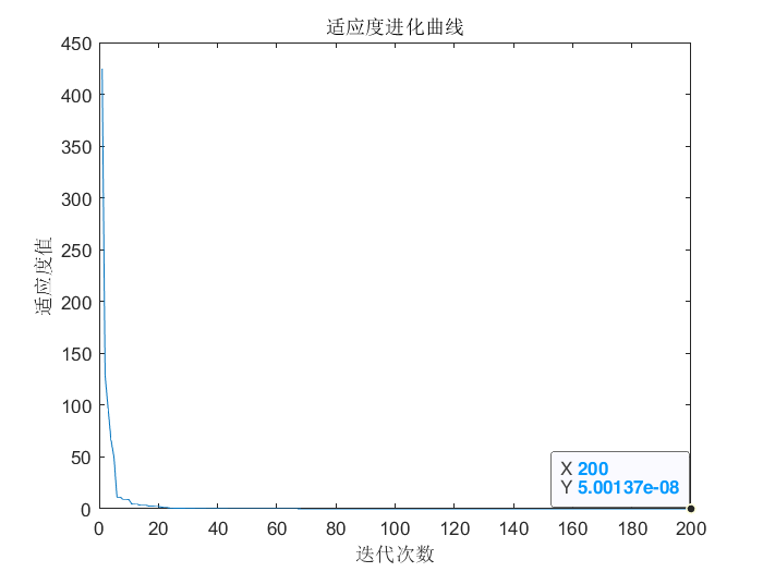
[find minimum] calculation function f ( x ) = ∑ i = 1 n x i 2 ( − 20 ≤ x i ≤ 20 ) f(x)=\sum_{i=1}^nx_{i}^2\quad(-20 \leq x_{i} \leq 20) f(x) = the minimum value of Σ i=1n xi2 (− 20 ≤ xi ≤ 20), where the dimension of individual x is n=10. This is a simple sum of squares function with only one minimum x = (0, 0,..., 0) and the theoretical minimum f (0, 0,..., 0) = 0

Solution: the simulation process is as follows:

(1) The number of initialization population particles is N=100, the particle dimension is D=10, the maximum number of iterations is T=200, the learning factor c1=c2=1.5, the inertia weight is w=0.8, and the maximum position is x m a x = 20 x_{max}=20 xmax = 20, position min x m i n = 20 x_{min}=20 xmin = 20, speed max v m a x = 10 v_{max}=10 vmax = 10, speed min v m i n = − 10 v_{min}=-10 vmin​=−10.

(2) Initialize the particle position x and velocity v of the population, the individual optimal position p and the optimal value pbest of the particle, and the global optimal position g and the optimal value gbest of the particle swarm.

(3) Update the position x and velocity v, and process the boundary conditions to judge whether to replace the optimal position of the individual particle p p p and optimal value p b e s t p_{best} pbest, particle swarm optimization, global optimal location g g g and optimal value g b e s t g_{best} gbest​​.

(4) Judge whether the termination conditions are met: If yes, the search process is ended and the optimization value is output; If not, continue iterative optimization.

After optimization, the fitness evolution curve is shown in the figure. The optimized result is x = [- 0.63250.1572 -0.4814 0.1091 -0.3154 0.2236 -0.3991 0.5907 0.0221 -0.1172] × 1 0 − 4 10^{-4} 10 − 4, function f ( x ) f(x) The minimum value of f(x) is 1.34 × 1 0 − 8 1.34×10^{-8} 1.34×10−8​.

MATLAB source program is as follows:

%%%%%%%%%%%%%%%%%Particle swarm optimization algorithm for function extremum%%%%%%%%%%%%%%%%%%%%%%%%%%
%%%%%%%%%%%%%%%%%%%%%%%%initialization%%%%%%%%%%%%%%%%%%%%%%%%%%%%%%%%%
clear all;              %Clear all variables
close all;              %Clear map
clc;                    %Clear screen
N=100;                  %Number of population particles
D=10;                   %Particle dimension
T=200;                  %Maximum number of iterations
c1=1.5;                 %Learning factor 1
c2=1.5;                 %Learning factor 2
w=0.8;                  %Inertia weight
Xmax=20;                %Position Max
Xmin=-20;               %Position min
Vmax=10;                %Maximum speed
Vmin=-10;               %Speed min
%%%%%%%%%%%%%%%%Initialize population individuals (limit position and speed)%%%%%%%%%%%%%%%%
x=rand(N,D) * (Xmax-Xmin)+Xmin;
v=rand(N,D) * (Vmax-Vmin)+Vmin;
%%%%%%%%%%%%%%%%%%Initialize individual optimal position and optimal value%%%%%%%%%%%%%%%%%%%
p=x;
pbest=ones(N,1);
for i=1:N
    pbest(i)=func1(x(i,:));
end
%%%%%%%%%%%%%%%%%%%Initialize global optimal location and optimal value%%%%%%%%%%%%%%%%%%
g=ones(1,D);
gbest=inf;
for i=1:N
    if(pbest(i)<gbest)
        g=p(i,:);
        gbest=pbest(i);
    end
end
gb=ones(1,T);
%%%%%%%%%%%Iterate successively according to the formula until the accuracy or iteration times are met%%%%%%%%%%%%%
for i=1:T
    for j=1:N
        %%%%%%%%%%%%%%Update individual optimal location and optimal value%%%%%%%%%%%%%%%%%
        if (func1(x(j,:))<pbest(j))
            p(j,:)=x(j,:);
            pbest(j)=func1(x(j,:));
        end
        %%%%%%%%%%%%%%%%Update global optimal location and optimal value%%%%%%%%%%%%%%%
        if(pbest(j)<gbest)
            g=p(j,:);
            gbest=pbest(j);
        end
        %%%%%%%%%%%%%%%%%Update position and speed values%%%%%%%%%%%%%%%%%%%%%
        v(j,:)=w*v(j,:)+c1*rand*(p(j,:)-x(j,:))...
            +c2*rand*(g-x(j,:));
        x(j,:)=x(j,:)+v(j,:);
        %%%%%%%%%%%%%%%%%%%%Boundary condition treatment%%%%%%%%%%%%%%%%%%%%%%
        for ii=1:D
            if (v(j,ii)>Vmax)  |  (v(j,ii)< Vmin)
                v(j,ii)=rand * (Vmax-Vmin)+Vmin;
            end
            if (x(j,ii)>Xmax)  |  (x(j,ii)< Xmin)
                x(j,ii)=rand * (Xmax-Xmin)+Xmin;
            end
        end
    end
    %%%%%%%%%%%%%%%%%%%%Record the historical global optimal value%%%%%%%%%%%%%%%%%%%%%
    gb(i)=gbest;
end
g;                         %Optimal individual         
gb(end);                   %optimal value
figure
plot(gb)
xlabel('Number of iterations');
ylabel('Fitness value');
title('Fitness evolution curve')
%%%%%%%%%%%%%%%%%%%Fitness function%%%%%%%%%%%%%%%%%%%%
function result=func1(x)
summ=sum(x.^2);
result=summ;
end

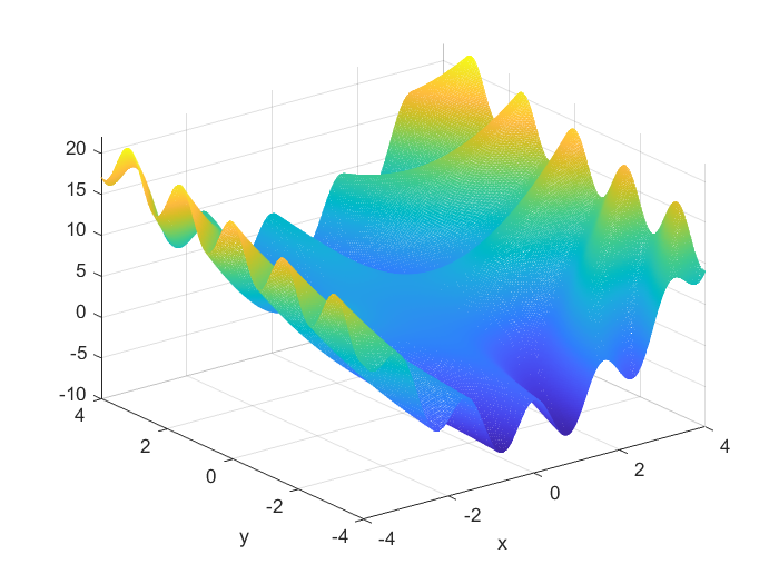
[find minimum] function f ( x , y ) = 3 c o s ( x y ) + x + y 2 f(x,y)=3cos(xy)+x+y^2 F (x, y) = the minimum value of 3cos (XY) + X + Y2, where the value range of X is [- 4,4], and the value range of Y is [- 4,4]. This is a function with multiple local extremums. The numerical graph of its function is shown in the figure. The MATLAB implementation program is as follows

%%%%%%%%%f(x，y)=3*cos(x*y)+x+y*y%%%%%%%%%%
clear all;              %Clear all variables
close all;              %Clear map
clc;                    %Clear screen
x=-4:0.02:4;
y=-4:0.02:4;
N=size(x,2);
for i=1:N
    for j=1:N
        z(i,j)=3*cos(x(i)*y(j))+x(i)+y(j)*y(j);
    end
end
mesh(x,y,z)
xlabel('x')
ylabel('y')

Solution: the simulation process is as follows:

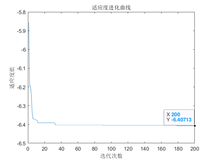
(1) The number of initialization population particles is N=100, the particle dimension is D=2, the maximum number of iterations is T=200, the learning factor c1=c2=1.5, and the maximum inertia weight is w m a x = 0.8 w_{max}=0.8 wmax = 0.8, the minimum inertia weight is w m i n = 0.4 w_{min}=0.4 wmin = 0.4, position max x m a x = 4 x_{max}=4 xmax = 4, position min x m i n = − 4 x_{min}=-4 xmin = − 4, speed max v m a x = 1 v_{max}=1 vmax = 1, speed min v m i n = − 1 v_{min}=-1 vmin​=−1.

(2) Initialize the particle position x and velocity v, the individual optimal position p and the optimal value pbest, the global optimal position g and the optimal value gbest.

(3) Calculate the dynamic inertia weight w, update the position x and velocity v, and process the boundary conditions to judge whether to replace the optimal position of the particle p p p and optimal value p b e s t p_{best} pbest, and the global optimal position of particle swarm optimization g g g and optimal value g b e s t g_{best} gbest​.

(4) Judge whether the termination conditions are met: If yes, the search process is ended and the optimization value is output; If not, continue iterative optimization

After optimization, the fitness evolution curve is shown in Figure 6.4. The optimized result is: when x=-4.0000 and y=-0.7578, the function f ( x ) f(x) f(x) obtain a minimum value of -6.408

MATLAB source program is as follows:

%%%%%%%%%%%%%%%%%Particle swarm optimization algorithm for function extremum%%%%%%%%%%%%%%%%%%%%%%%%%%
%%%%%%%%%%%%%%%%%%%%%%%%initialization%%%%%%%%%%%%%%%%%%%%%%%%%%%%%%%%%
clear all;              %Clear all variables
close all;              %Clear map
clc;                    %Clear screen
N=100;                  %Number of population particles
D=2;                    %Particle dimension
T=200;                  %Maximum number of iterations
c1=1.5;                 %Learning factor 1
c2=1.5;                 %Learning factor 2
Wmax=0.8;               %Maximum inertia weight
Wmin=0.4;               %Minimum inertia weight
Xmax=4;                 %Position Max
Xmin=-4;                %Position min
Vmax=1;                 %Maximum speed
Vmin=-1;                %Speed min
%%%%%%%%%%%%%%%%Initialize population individuals (limit position and speed)%%%%%%%%%%%%%%%%
x=rand(N,D) * (Xmax-Xmin)+Xmin;
v=rand(N,D) * (Vmax-Vmin)+Vmin;
%%%%%%%%%%%%%%%%%%Initialize individual optimal position and optimal value%%%%%%%%%%%%%%%%%%%
p=x;
pbest=ones(N,1);
for i=1:N
    pbest(i)=func2(x(i,:));
end
%%%%%%%%%%%%%%%%%%%Initialize global optimal location and optimal value%%%%%%%%%%%%%%%%%%
g=ones(1,D);
gbest=inf;
for i=1:N
    if(pbest(i)<gbest)
        g=p(i,:);
        gbest=pbest(i);
    end
end
gb=ones(1,T);
%%%%%%%%%%%Iterate successively according to the formula until the accuracy or iteration times are met%%%%%%%%%%%%%
for i=1:T
    for j=1:N
        %%%%%%%%%%%%%%Update individual optimal location and optimal value%%%%%%%%%%%%%%%%%
        if (func2(x(j,:))<pbest(j))
            p(j,:)=x(j,:);
            pbest(j)=func2(x(j,:));
        end
        %%%%%%%%%%%%%%%%Update global optimal location and optimal value%%%%%%%%%%%%%%%
        if(pbest(j)<gbest)
            g=p(j,:);
            gbest=pbest(j);
        end
        %%%%%%%%%%%%%%%%Calculate dynamic inertia weight value%%%%%%%%%%%%%%%%%%%%
        w=Wmax-(Wmax-Wmin)*i/T;
        %%%%%%%%%%%%%%%%%Update position and speed values%%%%%%%%%%%%%%%%%%%%%
        v(j,:)=w*v(j,:)+c1*rand*(p(j,:)-x(j,:))...
            +c2*rand*(g-x(j,:));
        x(j,:)=x(j,:)+v(j,:);
        %%%%%%%%%%%%%%%%%%%%Boundary condition treatment%%%%%%%%%%%%%%%%%%%%%%
        for ii=1:D
            if (v(j,ii)>Vmax)  |  (v(j,ii)< Vmin)
                v(j,ii)=rand * (Vmax-Vmin)+Vmin;
            end
            if (x(j,ii)>Xmax)  |  (x(j,ii)< Xmin)
                x(j,ii)=rand * (Xmax-Xmin)+Xmin;
            end
        end
    end
    %%%%%%%%%%%%%%%%%%%%Record the historical global optimal value%%%%%%%%%%%%%%%%%%%%%
    gb(i)=gbest;
end
g;                         %Optimal individual         
gb(end);                   %optimal value
figure
plot(gb)
xlabel('Number of iterations');
ylabel('Fitness value');
title('Fitness evolution curve')
%%%%%%%%%%%%%%%%%%%%%Fitness function%%%%%%%%%%%%%%%%%%%%%%%
function value=func2(x)
value=3*cos(x(1)*x(2))+x(1)+x(2)^2;
end

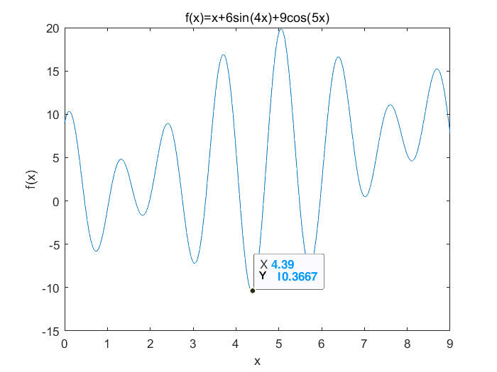
[find minimum] find the function with discrete particle swarm optimization algorithm f ( x ) = x + 6 s i n ( 4 x ) + 9 c o s ( 5 x ) f(x)=x+6sin(4x)+9cos(5x) F (x) = the minimum value of X + 6sin (4x) + 9cos (5x), where the value range of X is [0,9]. This is a function with multiple local extremums. Its function numerical graph is shown in the figure. Its MATLAB implementation program is as follows:

%%%%%%%%%f(x)=x+6sin(4x)+9cos(5x)%%%%%%%%%%
clear all;              %Clear all variables
close all;              %Clear map
clc;                    %Clear screen
x=0:0.01:9;
y=x+6*sin(4*x)+9*cos(5*x);
plot(x,y)
xlabel('x')
ylabel('f(x)')
title('f(x)=x+6sin(4x)+9cos(5x)')

Solution: the simulation process is as follows:

(1) The number of initialization population particles is N=100, the particle dimension is D=20, the maximum number of iterations is T=200, the learning factor c1=c2=1.5, and the maximum inertia weight is w m a x = 0.8 w_{max}=0.8 wmax = 0.8, the minimum inertia weight is w m i n = 0.4 w_{min}=0.4 wmin = 0.4, position max x m a x = 9 x_{max}=9 xmax = 9, position min x m i n = 0 x_{min}=0 xmin = 0, the maximum speed is v m a x = 10 v_{max}=10 vmax = 10, speed min v m i n = − 10 v_{min}=-10 vmin​=−10​​​.

(2) Initialize the velocity v and the binary coded population particle position x, calculate the fitness value, and obtain the individual optimal position p and the optimal value pbest, as well as the global optimal position g and the optimal value gbest.

(3) Calculate the dynamic inertia weight w, update the position x and velocity v, and process the boundary conditions to judge whether to replace the optimal position of the particle p p p and optimal value p b e s t p_{best} pbest, and the global optimal position of particle swarm optimization g g g and optimal value g b e s t g_{best} gbest​.

(4) Judge whether the termination conditions are met: If yes, the search process is ended and the optimization value is output; If not, continue iterative optimization.

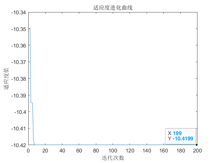
The fitness evolution curve is shown in the figure. The optimized result is: when x=4.37, the function f ( x ) f(x) f(x) obtain a minimum value of -10.42.

MATLAB source program is as follows:

%%%%%%%%%%%%%%%%%Discrete particle swarm optimization algorithm for function extremum%%%%%%%%%%%%%%%%%%%%%%%
%%%%%%%%%%%%%%%%%%%%%%%%initialization%%%%%%%%%%%%%%%%%%%%%%%%%%%%%%%%%
clear all;              %Clear all variables
close all;              %Clear map
clc;                    %Clear screen
N=100;                  %Number of population particles
D=20;                   %Particle dimension
T=200;                  %Maximum number of iterations
c1=1.5;                 %Learning factor 1
c2=1.5;                 %Learning factor 2
Wmax=0.8;               %Maximum inertia weight
Wmin=0.4;               %Minimum inertia weight
Xs=9;                   %Position Max
Xx=0;                   %Position min
Vmax=10;                %Maximum speed
Vmin=-10;               %Speed min
%%%%%%%%%%%%%%%%Initialize population individuals (limit position and speed)%%%%%%%%%%%%%%%%
x=randi([0,1],N,D);        %The binary coded initial population is obtained randomly
v=rand(N,D) * (Vmax-Vmin)+Vmin;
%%%%%%%%%%%%%%%%%%Initialize individual optimal position and optimal value%%%%%%%%%%%%%%%%%%%
p=x;
pbest=ones(N,1);
for i=1:N
    pbest(i)= func3(x(i,:),Xs,Xx);
end
%%%%%%%%%%%%%%%%%%%Initialize global optimal location and optimal value%%%%%%%%%%%%%%%%%%
g=ones(1,D);
gbest=inf;
for i=1:N
    if(pbest(i)<gbest)
        g=p(i,:);
        gbest=pbest(i);
    end
end
gb=ones(1,T);
%%%%%%%%%%%Iterate successively according to the formula until the accuracy or iteration times are met%%%%%%%%%%%%%
for i=1:T
    for j=1:N
        %%%%%%%%%%%%%%Update individual optimal location and optimal value%%%%%%%%%%%%%%%%%
        if (func3(x(j,:),Xs,Xx)<pbest(j))
            p(j,:)=x(j,:);
            pbest(j)=func3(x(j,:),Xs,Xx);
        end
        %%%%%%%%%%%%%%%%Update global optimal location and optimal value%%%%%%%%%%%%%%%
        if(pbest(j)<gbest)
            g=p(j,:);
            gbest=pbest(j);
        end
        %%%%%%%%%%%%%%%%Calculate dynamic inertia weight value%%%%%%%%%%%%%%%%%%%%
        w=Wmax-(Wmax-Wmin)*i/T;
        %%%%%%%%%%%%%%%%%Update position and speed values%%%%%%%%%%%%%%%%%%%%%
        v(j,:)=w*v(j,:)+c1*rand*(p(j,:)-x(j,:))...
            +c2*rand*(g-x(j,:));
        %%%%%%%%%%%%%%%%%%%%Boundary condition treatment%%%%%%%%%%%%%%%%%%%%%%
        for ii=1:D
            if (v(j,ii)>Vmax)  |  (v(j,ii)< Vmin)
                v(j,ii)=rand * (Vmax-Vmin)+Vmin;
            end
        end    
        vx(j,:)=1./(1+exp(-v(j,:)));
        for jj=1:D
            if vx(j,jj)>rand
                x(j,jj)=1;
            else
                x(j,jj)=0;
            end
        end      
    end
    %%%%%%%%%%%%%%%%%%%%Record the historical global optimal value%%%%%%%%%%%%%%%%%%%%%
    gb(i)=gbest;
end
g;                       %Optimal individual 
m=0;
for j=1:D
    m=g(j)*2^(j-1)+m;
end
f1=Xx+m*(Xs-Xx)/(2^D-1); %optimal value
figure
plot(gb)
xlabel('Number of iterations');
ylabel('Fitness value');
title('Fitness evolution curve')
%%%%%%%%%%%%%%%%%%%%%%%%%Fitness function%%%%%%%%%%%%%%%%%%%%%%%%%%%%
function result=func3(x,Xs,Xx)
m=0;
D=length(x);
for j=1:D
    m=x(j)*2^(j-1)+m;
end
f=Xx+m*(Xs-Xx)/(2^D-1);            %Decode to decimal
fit= f+6*sin(4*f)+9*cos(5*f);
result=fit;
end

[1] Bao Ziyang, Yu Jizhou, Yang Bin. Intelligent optimization algorithm and its MATLAB example [M] Electronic Industry Press, 2021