1, Introduction
1 Introduction
Modulation: the message signal is placed on a certain parameter of the carrier to form a modulated signal.
Demodulation: the inverse process of modulation to recover the message signal from the modulated signal.
2 purpose of modulation
In wireless communication, matching channel characteristics, increasing the frequency of transmitted signal and reducing the size of antenna; Spectrum shifting, simultaneous transmission of multiple signals in one channel, multiplexing and improving channel utilization; Expand the signal bandwidth and improve the anti-interference ability of the system; Realize the exchange of bandwidth and signal-to-noise ratio (effectiveness and reliability); It is necessary to translate analog / digital signals to connect PC to Internet by telephone line.
3 Classification of modulation
3.1 signals involved
Message signal, also known as modulation signal and baseband signal;
Carrier: carrier, commonly used sine wave and pulse sequence;
Modulated signal: modulated carrier, which carries the information of message signal and has various forms.
3.2 it can be classified from different angles
According to the type of modulation signal: analog modulation / digital modulation
According to the spectrum structure of modulated signal: linear modulation / nonlinear modulation
Modulated parameters according to sinusoidal carrier: amplitude modulation / frequency modulation / phase modulation
According to the type of carrier signal: continuous wave modulation / pulse modulation
4 amplitude modulation
4.1 General Model
(1) Theoretical basis: Fourier transform
(2) General model
Amplitude modulation: the message signal controls the amplitude of the sinusoidal carrier.
Methods: the message signal is multiplied by the carrier signal through the multiplier, and then through the band-pass filter (time-domain convolution filter characteristics).
Examples: AM, DSB, SSB, VSB.
4.2 conventional double sideband AM
t domain: waveform of modulated signal, modulation / demodulation method
f domain: spectrum of modulated signal, bandwidth B
The envelope of AM signal is proportional to the law of message signal, so a simple * * envelope detection method (incoherent demodulation) * * demodulation can be used;
The spectrum consists of carrier, upper sideband USB and lower sideband LSB. Bandwidth BAM=2fH;
Amplitude modulation is also called linear modulation;
Application: medium and short wave AM broadcasting.
Disadvantages: low power utilization, up to 50%
4.3 suppression of carrier double sideband DSB
The spectrum is composed of upper sideband USB and lower sideband LSB without carrier component. Bandwidth BDSB=BAM=2fH;
The modulation efficiency can reach 100%.
Coherent demodulation:
Methods: the message signal is multiplied by the coherent carrier signal through the multiplier, and then through the low-pass filter (time-domain convolution filter characteristics).
Requirements: carrier synchronization (coherent carrier and carrier signal are in the same frequency and phase)
4.4 SSB modulation
Only one sideband is transmitted, and the frequency band utilization is high. Bandwidth BSSB=BAM/2=fH; In spectrum crowded communication occasions, such as short wave communication and multi-channel carrier telephone system. Low power consumption characteristics. Used in mobile communication system.
Disadvantages: the equipment is complex, there are technical difficulties, and coherent demodulation is required.
4.5 residual sideband modulation VSB
Characteristics of residual sideband filter: complementary symmetry at carrier frequency; A scheme between single sideband and double sideband.
5 angle modulation
Sinusoidal carrier has three parameters: amplitude, frequency and phase. Can carry message signals.
Both frequency (FM) and phase (PM) are called angle modulation.
Frequency modulation (FM)
When the amplitude is constant, the instantaneous phase is differentiated by t to obtain the instantaneous angular frequency.
The frequency spectrum of FM consists of numerous pairs of side frequencies wc ± nwm on both sides of the carrier frequency component wc, and its amplitude depends on mf;
Theoretically, the bandwidth of FM is infinite;
In practice, the FM bandwidth is calculated by Carson formula: BFM=2(mf+1)fm. FM is the highest frequency of the modulated signal
FM modulation is nonlinear modulation. FM demodulation, also known as frequency discrimination, is realized by differential circuit + envelope detection.
Characteristics and application of FM
Features: constant amplitude and constant envelope.
Advantages: strong anti noise ability;
Cost: occupy large channel bandwidth and low spectrum utilization;
Application: occasions with high quality or high channel noise. Such as satellite communication, mobile communication, microwave communication, etc.
6 anti noise performance
Performance index: output signal-to-noise ratio, system gain
Input SNR: Ni=n0B. n0 is the unilateral power spectral density of noise, B=2fH is the bandwidth, which is twice the baseband bandwidth.
AM DSB SSB VSB (amplitude modulation)
Coherent demodulator: linear demodulation, signal and noise can be processed separately.
The anti noise performance of double sideband and single sideband modulation is the same.
When the signal-to-noise ratio is small, the signal is interfered into noise, resulting in threshold effect. The reason is the nonlinear demodulation of envelope detection.
The signal-to-noise ratio is fixed.
FM (angle modulation)
FM system can improve anti noise performance (signal-to-noise ratio) by increasing transmission bandwidth.
summary
Spectrum utilization SSB > VSB > DSB / am > FM
Anti noise performance: FM > DSB / SSB > VSB > am
Equipment complexity: AM is the simplest, DSB/FM is the second, and SSB is the most complex
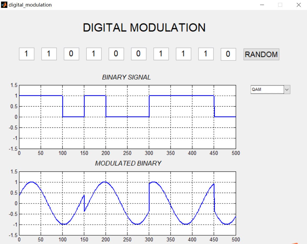
2, Partial source code
function varargout = digital_modulation(varargin)
%DIGITAL_MODULATION
% Begin initialization code - DO NOT EDIT
gui_Singleton = 1;
gui_State = struct('gui_Name', mfilename, ...
'gui_Singleton', gui_Singleton, ...
'gui_OpeningFcn', @digital_modulation_OpeningFcn, ...
'gui_OutputFcn', @digital_modulation_OutputFcn, ...
'gui_LayoutFcn', [] , ...
'gui_Callback', []);
if nargin && ischar(varargin{1})
gui_State.gui_Callback = str2func(varargin{1});
end
if nargout
[varargout{1:nargout}] = gui_mainfcn(gui_State, varargin{:});
else
gui_mainfcn(gui_State, varargin{:});
end
% End initialization code - DO NOT EDIT
% --- Executes just before digital_modulation is made visible.
function digital_modulation_OpeningFcn(hObject, eventdata, handles, varargin)
% This function has no output args, see OutputFcn.
% hObject handle to figure
% eventdata reserved - to be defined in a future version of MATLAB
% handles structure with handles and user data (see GUIDATA)
% varargin command line arguments to digital_modulation (see VARARGIN)
hold off;
axes(handles.axes1);
h=[1 1 0 1 0 0 1 1 1 0];
hold off;
bit=[];
for n=1:2:length(h)-1;
if h(n)==0 & h(n+1)==1
se=[zeros(1,50) ones(1,50)];
elseif h(n)==0 & h(n+1)==0
se=[zeros(1,50) zeros(1,50)];
elseif h(n)==1 & h(n+1)==0
se=[ones(1,50) zeros(1,50)];
elseif h(n)==1 & h(n+1)==1
se=[ones(1,50) ones(1,50)];
end
bit=[bit se];
end
plot(bit,'LineWidth',1.5);grid on;
axis([0 500 -1.5 1.5]);
%*-*-*-*-*-*-*-*-*-*-*-*-*-*-*-*-*-*-*-*-*-*-
axes(handles.axes3)
hold off;
fc=30;
g=[1 1 0 1 0 0 1 1 1 0]; %modulante
n=1;
while n<=length(g)
if g(n)==0
tx=(n-1)*0.1:0.1/100:n*0.1;
p=(1)*sin(2*pi*fc*tx);
plot(tx,p,'LineWidth',1.5);grid on;
hold on;
else
tx=(n-1)*0.1:0.1/100:n*0.1;
p=(2)*sin(2*pi*fc*tx);
plot(tx,p,'LineWidth',1.5);grid on;
hold on;
end
n=n+1;
end
% Choose default command line output for digital_modulation
handles.output = hObject;
% Update handles structure
guidata(hObject, handles);
% UIWAIT makes digital_modulation wait for user response (see UIRESUME)
% uiwait(handles.figure1);
% --- Outputs from this function are returned to the command line.
function varargout = digital_modulation_OutputFcn(hObject, eventdata, handles)
% varargout cell array for returning output args (see VARARGOUT);
% hObject handle to figure
% eventdata reserved - to be defined in a future version of MATLAB
% handles structure with handles and user data (see GUIDATA)
% Get default command line output from handles structure
varargout{1} = handles.output;
% --- Executes on button press in random.
function random_Callback(hObject, eventdata, handles)
% hObject handle to random (see GCBO)
% eventdata reserved - to be defined in a future version of MATLAB
% handles structure with handles and user data (see GUIDATA)
a=round(rand(1,10)); %genarar bits aleatorios
ran=[a(1),a(2),a(3),a(4),a(5),a(6),a(7),a(8),a(9),a(10)];
set(handles.bit1,'String',ran(1));
set(handles.bit2,'String',ran(2));
set(handles.bit3,'String',ran(3));
set(handles.bit4,'String',ran(4));
set(handles.bit5,'String',ran(5));
set(handles.bit6,'String',ran(6));
set(handles.bit7,'String',ran(7));
set(handles.bit8,'String',ran(8));
set(handles.bit9,'String',ran(9));
set(handles.bit10,'String',ran(10));
%*-*-*-*-*-*-*-*-*-*-*-*-*-*-*-*-*-*-*-*-*-*
handles.bits=ran;
h=handles.bits;
axes(handles.axes1)
hold off;
bit=[];
for n=1:2:length(h)-1;
if h(n)==0 & h(n+1)==1
se=[zeros(1,50) ones(1,50)];
elseif h(n)==0 & h(n+1)==0
se=[zeros(1,50) zeros(1,50)];
elseif h(n)==1 & h(n+1)==0
se=[ones(1,50) zeros(1,50)];
elseif h(n)==1 & h(n+1)==1
se=[ones(1,50) ones(1,50)];
end
bit=[bit se];
end
plot(bit,'LineWidth',1.5);grid on;
axis([0 500 -1.5 1.5]);
%*-*-*-*-*-*-*-*-*-*-*-*-
hold off;
axes(handles.axes3);
cod=get(handles.select_mod,'Value');
switch cod
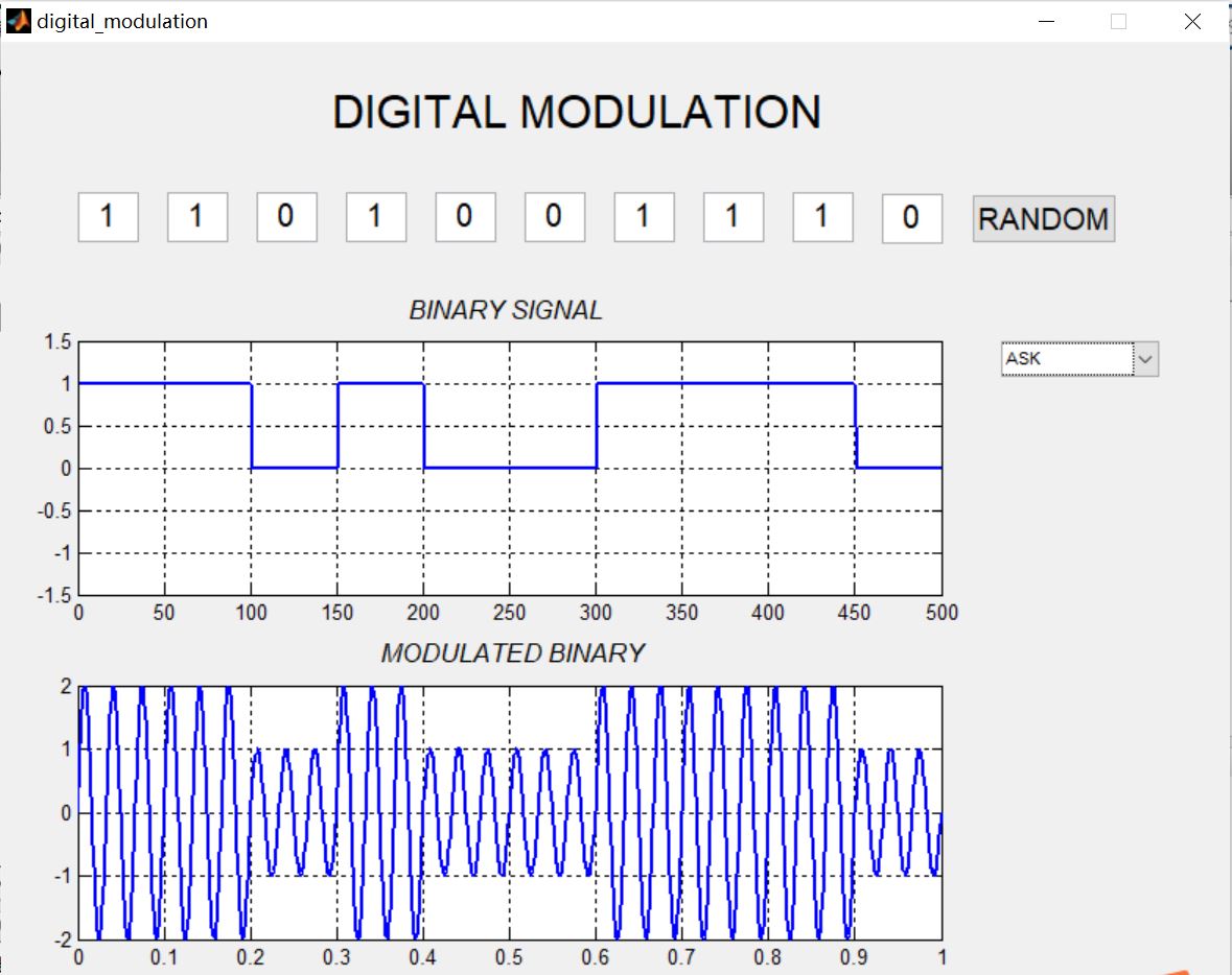
%*-*-*-*Modulation ASK*-*-*-*-*-*-*-*-*
case 1
hold off;
axes(handles.axes3)
fc=30;
g=handles.bits; %modulante
n=1;
while n<=length(g)
if g(n)==0
tx=(n-1)*0.1:0.1/100:n*0.1;
p=(1)*sin(2*pi*fc*tx);
plot(tx,p,'LineWidth',1.5);grid on;
hold on;
% axis([0 n*2/fc -3 3]);
else
tx=(n-1)*0.1:0.1/100:n*0.1;
p=(2)*sin(2*pi*fc*tx);
plot(tx,p,'LineWidth',1.5);grid on;
hold on;
end
n=n+1;
end
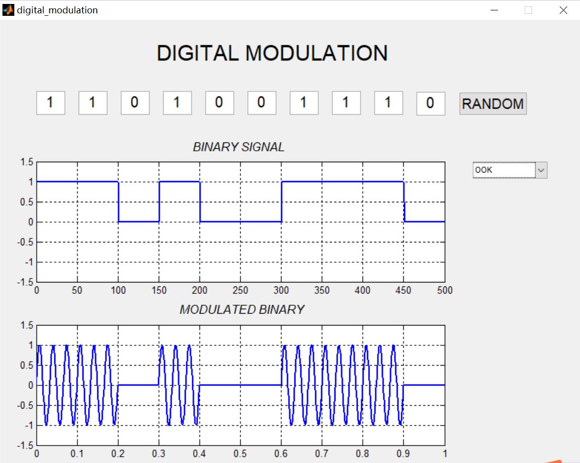
%*-*-*-*-*-*-*-Modulation OOK*-*-*-*-*-*-*-*-*-
case 2
hold off;
axes(handles.axes3);
t=0:0.001:1;
m=1;
fc=30;
g=handles.bits; %modulante
n=1;
while n<=length(g)
tx=(n-1)*1/length(g):0.001:n*1/length(g);
p=(g(n))*sin(2*pi*fc*tx);
plot(tx,p,'LineWidth',1.5);
hold on;
axis([0 (n)*1/length(g) -1.5 1.5]);
grid on;
n=n+1;
end
%*-*-*-*-*-*-*-Modulation BPSK*-*-*-*-*-*-*-*-*-*-*-
case 3
axes(handles.axes3)
hold off;
g=handles.bits;
fc=10;
n=1;
while n<=length(g)
if g(n)==0 %0 is -1
tx=(n-1)*0.1:0.1/100:n*0.1;
p=(-1)*sin(2*pi*fc*tx);
plot(tx,p,'LineWidth',1.5);grid on;
hold on;
else
tx=(n-1)*0.1:0.1/100:n*0.1;
p=(1)*sin(2*pi*fc*tx);
plot(tx,p,'LineWidth',1.5);grid on;
hold on;
end
n=n+1;
end
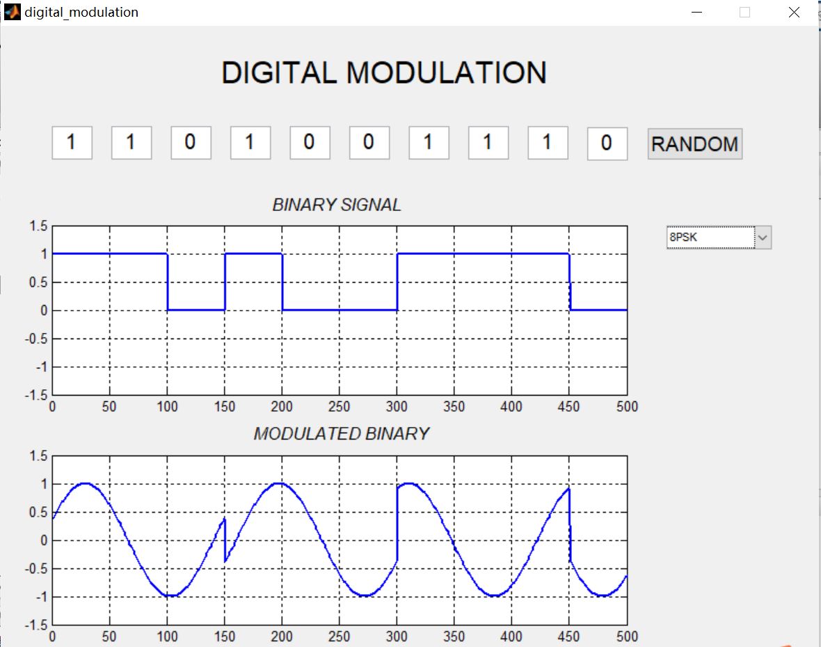
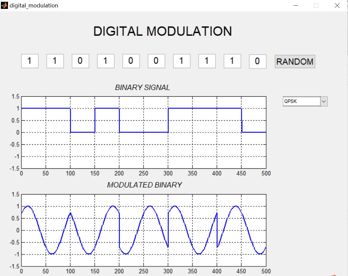
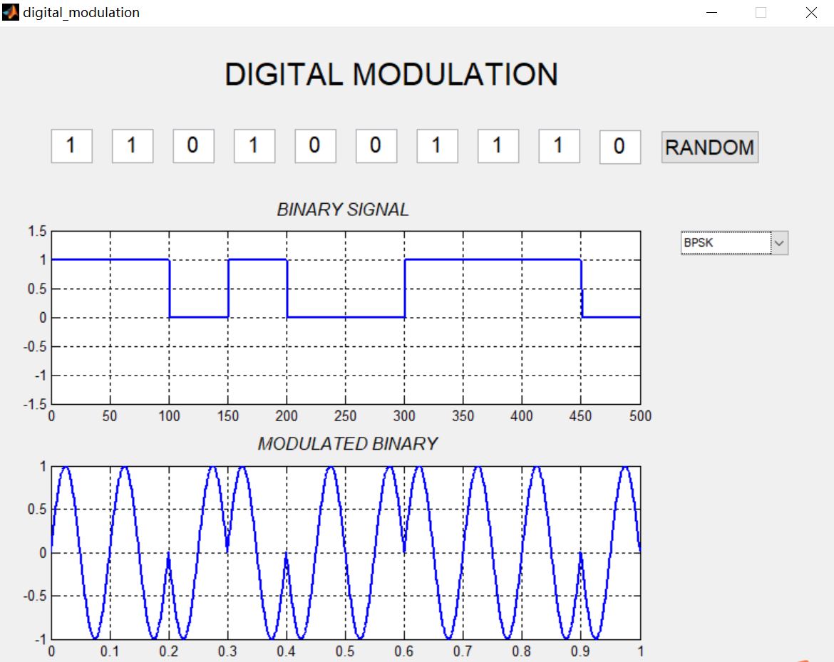
3, Operation results
4, matlab version and references
1 matlab version
2014a
2 references
[1] Shen Zaiyang. Proficient in MATLAB signal processing [M]. Tsinghua University Press, 2015
[2] Gao Baojian, Peng Jinye, Wang Lin, pan Jianshou. Signal and system -- Analysis and implementation using MATLAB [M]. Tsinghua University Press, 2020
[3] Wang Wenguang, Wei Shaoming, Ren Xin. MATLAB implementation of signal processing and system analysis [M]. Electronic Industry Press, 2018