1, Introduction to SIFT registration

SIFT, scale invariant feature transformation, is a description used in the field of image processing. This description has scale invariance and can detect key points in the image. It is a local feature descriptor.
1. SIFT algorithm features:
(1) It has good stability and invariance, can adapt to the changes of rotation, scale scaling and brightness, and can be free from the interference of angle change, affine transformation and noise to a certain extent.
(2) It has good discrimination and can match the discrimination information quickly and accurately in the massive feature database
(3) Multiplicity, even if there is only a single object, can produce a large number of eigenvectors
(4) High speed, fast feature vector matching
(5) Scalability, can be combined with other forms of eigenvectors

2 essence of SIFT algorithm
Find the key points in different scale spaces, and calculate the direction of the key points.

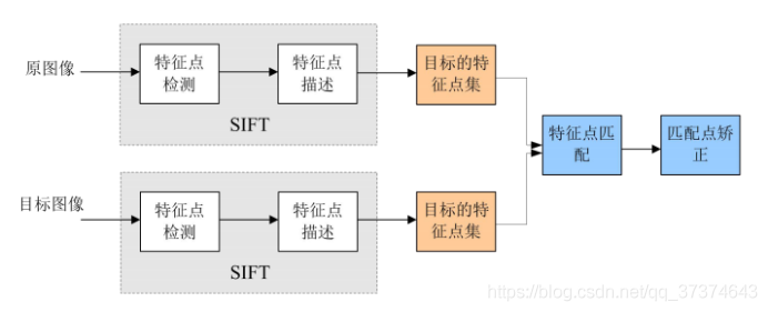
3. The SIFT algorithm realizes feature matching mainly in the following three processes:
(1) Extract key points: key points are some very prominent points that will not disappear due to lighting, scale, rotation and other factors, such as corner points, edge points, bright spots in dark areas and dark spots in bright areas. This step is to search for image positions in all scale spaces. Gaussian differential function is used to identify potential points of interest with scale and rotation invariance.
(2) Locate the key points and determine the feature direction: at each candidate position, a fine fitting model is used to determine the position and scale. The selection of key points depends on their stability. Then, one or more directions are assigned to each key position based on the local gradient direction of the image. All subsequent operations on image data are transformed relative to the direction, scale and position of key points, so as to provide invariance to these transformations.
(3) By comparing the feature vectors of each key point, several pairs of matching feature points are found, and the corresponding relationship between scenes is established.

4 scale space
(1) Concept
Scale space is the concept and method of trying to simulate human eyes to observe objects in the field of images. For example, when observing a tree, the key is whether we want to observe the leaves or the whole tree: if it is a whole tree (equivalent to observing in a large scale), the details of the image should be removed. If it is a leaf (observed at a small scale), the local details should be observed.
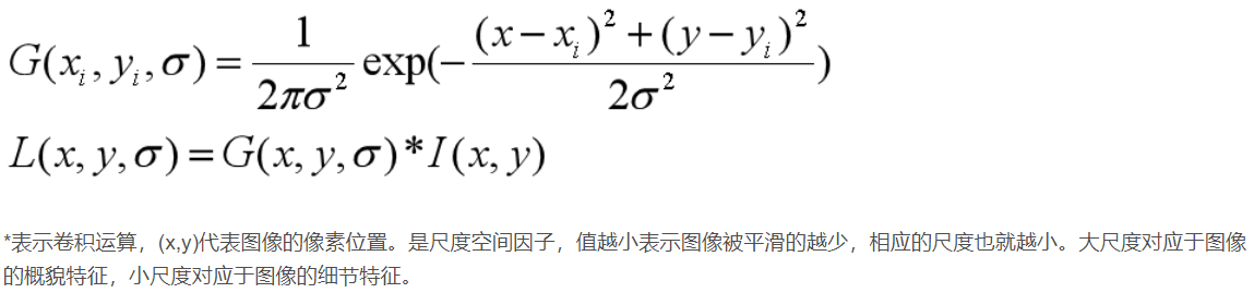
SIFT algorithm adopts Gaussian kernel function to filter when constructing scale space, so that the original image can save the most detailed features. After Gaussian filtering, the detailed features are gradually reduced to simulate the feature representation in the case of large scale.
There are two main reasons for filtering with Gaussian kernel function:
a Gaussian kernel function is the only scale invariant kernel function.
b DoG kernel function can be approximated as LoG function, which can make feature extraction easier. At the same time, the author David Lowe proposed in the paper that filtering after twice up sampling the original image can retain more information for subsequent feature extraction and matching. In fact, scale space image generation is the current image and different scale kernel parameters σ The image generated after convolution operation.
(2) Show
L(x, y, σ) , It is defined as the original image I(x, y) and a variable scale 2-dimensional Gaussian function G(x, y, σ) Convolution operation.

5 construction of Gaussian pyramid
(1) Concept
The scale space is represented by Gaussian pyramid during implementation. The construction of Gaussian pyramid is divided into two steps:
a Gaussian smoothing of the image;
b downsampling the image.

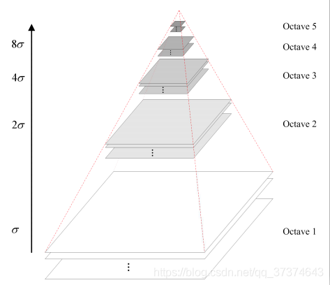
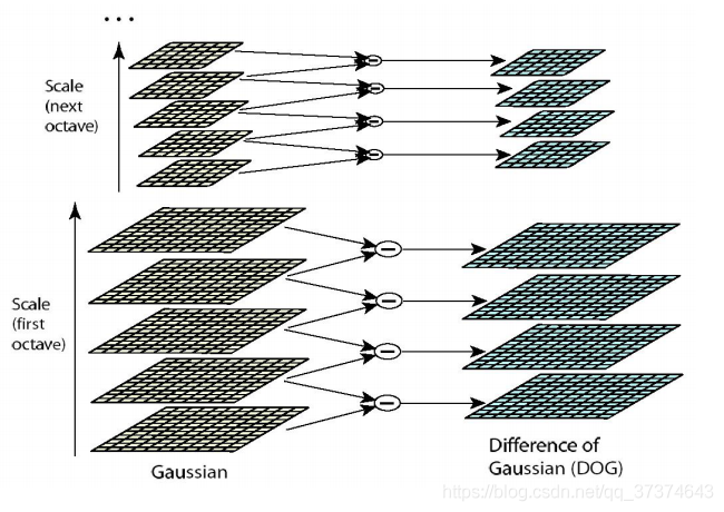
The pyramid model of image refers to the pyramid model in which the original image is continuously reduced and sampled to obtain a series of images of different sizes, from large to small, from bottom to top. The original image is the first layer of the gold tower, and the new image obtained by each down sampling is one layer of the pyramid (one image per layer) , each pyramid has n layers in total. In order to make the scale reflect its continuity, the Gaussian pyramid adds Gaussian filtering on the basis of simple downsampling. As shown in the above figure, Gaussian blur is used for an image in each layer of the image pyramid with different parameters, Octave represents the number of image groups that can be generated by an image, and Interval represents the number of image layers included in a group of images. In addition, during downsampling , the initial image (bottom image) of a group of images on the Gaussian pyramid is obtained by sampling every other point of the penultimate image of the previous group of images.
(2) Show
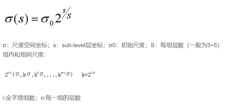
If there are o groups and s layers in the Gaussian image pyramid, there are

6 DOG space extreme value detection
(1) DOG function

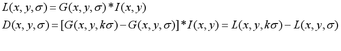
(2) DoG Gaussian difference pyramid
a corresponding to the DOG operator, the DOG pyramid needs to be constructed.
The change of pixel value on the image can be seen through the Gaussian difference image. (if there is no change, there is no feature. The feature must be as many points as possible.) the DOG image depicts the contour of the target.

B. dog local extreme value detection
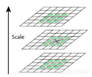
Feature points are composed of local extreme points in dog space. In order to find the extreme points of dog function, each pixel point shall be compared with all its adjacent points to see whether it is larger or smaller than its adjacent points in image domain and scale domain. Feature points are composed of local extreme points in dog space. In order to find the extreme points of dog function, each pixel point shall be compared with all its adjacent points Compare it to see if it is larger or smaller than the adjacent points in its image domain and scale domain. As shown in the figure below, the middle detection point corresponds to 8 adjacent points in the same scale and 9 adjacent points in the upper and lower scales × The two points are compared with 26 points in total to ensure that extreme points are detected in both scale space and two-dimensional image space.

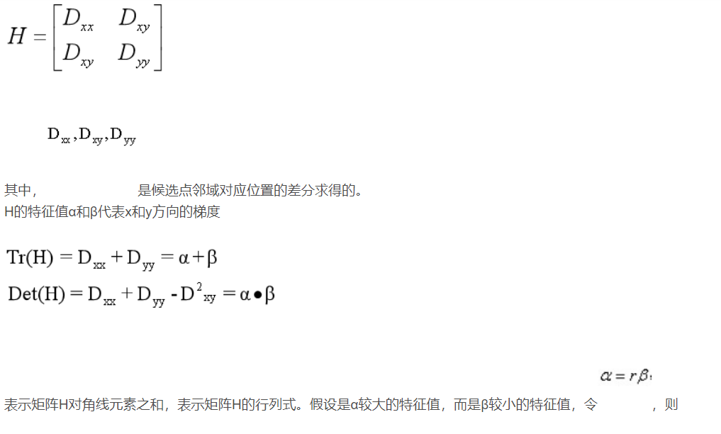
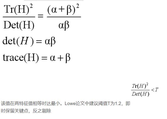
b remove edge effects
The principal curvature value is larger in the direction of edge gradient, but smaller along the edge direction. The principal curvature of DoG function D(x) of candidate feature points is the same as 2 × 2Hessian matrix is proportional to the eigenvalue of H.


7 key point direction assignment
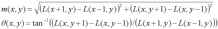
(1) To find the extreme points through scale invariance, it is necessary to assign a reference direction to each key point by using the local features of the image, so that the descriptor is invariant to the image rotation. For the key points detected in the DOG pyramid, collect the Gaussian pyramid image 3 σ The gradient and direction distribution characteristics of pixels in the neighborhood window. The modulus and direction of the gradient are as follows:

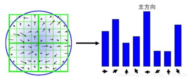
(2) This algorithm uses the gradient histogram statistical method, takes the key points as the origin, and determines the direction of the key points according to the image pixels in a certain area. After completing the gradient calculation of key points, histogram is used to count the gradient and direction of pixels in the neighborhood. The gradient histogram divides the direction range of 0 ~ 360 degrees into 36 columns, of which each column is 10 degrees. As shown in the figure below, the peak direction of the histogram represents the main direction of the key point, the peak direction of the histogram represents the direction of the neighborhood gradient at the feature point, and the maximum value in the histogram is taken as the main direction of the key point. In order to enhance the robustness of matching, only the direction whose peak value is greater than 80% of the peak value in the main direction is retained as the secondary direction of the key point.

8 key point description
For each key point, it has three information: location, scale and direction. Create a descriptor for each key point and describe the key point with a set of vectors so that it does not change with various changes, such as illumination change, viewing angle change, etc. This descriptor includes not only the key points, but also the pixels around the key points that contribute to it, and the descriptor should have high uniqueness to improve the probability of correct matching of feature points.

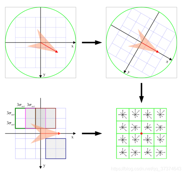
Lowe experimental results show that the descriptor adopts 4 × four × 8 = 128 dimensional vector representation, the comprehensive effect is the best (invariance and uniqueness).

9 key point matching
(1) For template map (reference image) and real-time map (observation map,
observation image) creates a subset of key descriptions. Target recognition is accomplished by comparing the key point descriptors in the two-point set. The similarity measure of key descriptor with 128 dimensions adopts Euclidean distance.
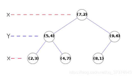
(3) Matching can be completed by exhaustive method, but it takes too much time. Therefore, the data structure of kd tree is generally used to complete the search. The search content is to search the original image feature points closest to the feature points of the target image and the sub adjacent original image feature points based on the key points of the target image.
Kd tree, as shown below, is a balanced binary tree

10 summary
SIFT features have stability and invariance, and play a very important role in the field of image processing and computer vision. It is also very complex. Because it is not long to contact sift, we still do not understand the relevant knowledge. After consulting and referring from many parties, the content of this article is not detailed enough. Please forgive me. The following is a rough summary of SIFT algorithm.
(1) Extreme value detection in DoG scale space.
(2) Delete unstable extreme points.
(3) Determine the main direction of feature points
(4) The descriptor of feature points is generated for key point matching.

2, Partial source code

%Image Stitching assignment

img1=imread('1.jpg');

%set this image as the reference image.
ref_img2=imread('2.jpg');

img3=imread('3.jpg');

% find homography between img1 and ref image img2
%use harris and stephens corner detector to get the loacl features of the image.
[ref_a,ref_b,ref_c]=harris(ref_img2);
[a1,b1,c1]=harris(img1);
[a2,b2,c2]=harris(img3);
% now use the SIFT decriptor to get the descriptors of both the image 
% Only scale invariant not rotational invariant. Not needed for this
% assignment.
%find circles for ref and img_1
%radius of ref_img
radius_ref=repmat(3,[size(ref_c),1]);
%radius of img_1;
radius_img1=repmat(3,[size(c1),1]);
%radius of img3
radius_img3=repmat(3,[size(c2),1]);
%create a circle array of N*3 size for repmat


%use sift descriptors
sift_desc_ref=find_sift(ref_img2,ref_circle,2);
sift_desc_img1=find_sift(img1,img1_circle,2);
sift_desc_img2=find_sift(img3,img3_circle,2);   
%Match features between two images.
%use the dist2 function two find the 2-nearest neighbors
dist_ref_img1=dist2(sift_desc_ref,sift_desc_img1);
dist_ref_img2=dist2(sift_desc_ref,sift_desc_img2);

[row, col]=size(dist_ref_img1);
[row1, col1]=size(dist_ref_img2);
%function for matching
[img_ref,image_cores]=matching_features(row,dist_ref_img1,ref_circle,img1_circle,img1);
[img_ref1,image_cores1]=matching_features(row1,dist_ref_img2,ref_circle,img3_circle,img3);
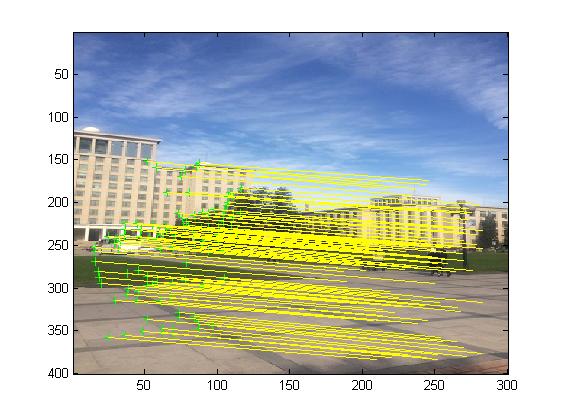
%Plot correspondence
PlotImageCores(img_ref,image_cores,img1);
PlotImageCores(img_ref1,image_cores1,img3);

%Use Ransac to get good amount of inliners.
inliners=RANSAC(img_ref,image_cores);
inliners1=RANSAC(img_ref1,image_cores1);
%Find inliner points for the image
[final_inliner_ref,final_inliner_img]=InlierPoint(img_ref,image_cores,inliners);
[final_inliner_ref1,final_inliner_img1]=InlierPoint(img_ref1,image_cores1,inliners1);

%Plot new inliner correspondence

H_re1=computeH(final_inliner_ref1,final_inliner_img1);
%reproject on the image and do the image stitching 
final_mosaic=Mosaicing(ref_img2,img1,H_re);
final_mosaic=uint8(final_mosaic);
final_mosaic1=Mosaicing(ref_img2,img3,H_re1);
final_mosaic1=uint8(final_mosaic1);
final_image=Mosaicing(final_mosaic,final_mosaic1,eye(3));
[rowF,colF,K]=size(final_mosaic);
final_image=zeros(rowF,colF,3);
for i=1:rowF
    for j=1:colF
        for k=1:K
            if final_mosaic(i,j,k)>final_mosaic1(i,j,k)
                final_image(i,j,k)=final_mosaic(i,j,k);
            elseif final_mosaic(i,j,k)<final_mosaic1(i,j,k)
                final_image(i,j,k)=final_mosaic1(i,j,k);
            elseif final_mosaic(i,j,k)==final_mosaic1(i,j,k)
                final_image(i,j,k)=final_mosaic(i,j,k);
            end
        end
    end
end
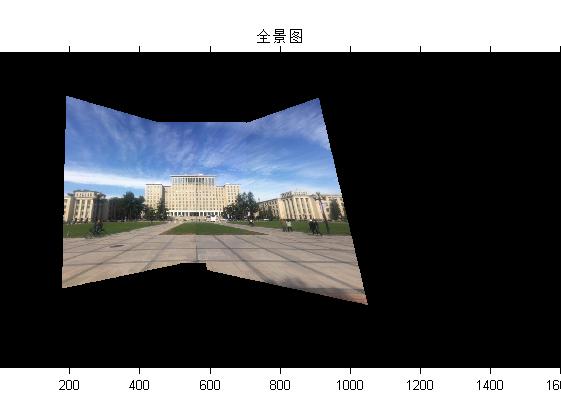
figure;
imshow(uint8(final_image),'InitialMagnification','fit');
title('Panorama');



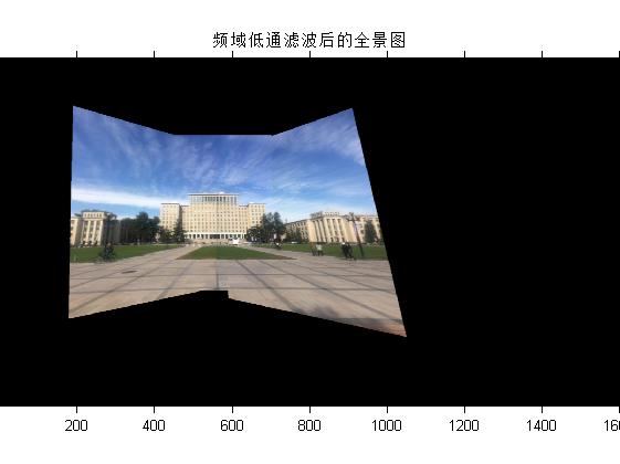
figure;
imshow(uint8(final_image),'InitialMagnification','fit');
title('Panorama after frequency domain low-pass filtering');
function sift_arr = find_sift(I, circles, enlarge_factor)
%%
%% Compute non-rotation-invariant SIFT descriptors of a set of circles 
%% I is the image
%% circles is an Nx3 array where N is the number of circles, where the
%%    first column is the x-coordinate (column), the second column is the y-coordinate (row),
%%    and the third column is the radius
%% enlarge_factor is by how much to enarge the radius of the circle before
%%    computing the descriptor (a factor of 1.5 or larger is usually necessary
%%    for best performance)
%% The output is an Nx128 array of SIFT descriptors
%% (c) Lana Lazebnik
%%

if ndims(I) == 3
    I = im2double(rgb2gray(I));
else
    I = im2double(I);
end


fprintf('Running find_sift\n');

% parameters (default SIFT size)
num_angles = 8;
num_bins = 4;
num_samples = num_bins * num_bins;
alpha = 9; % smoothing for orientation histogram

if nargin < 3
    enlarge_factor = 1.5;
end

angle_step = 2 * pi / num_angles;
angles = 0:angle_step:2*pi;
angles(num_angles+1) = []; % bin centers

[hgt wid] = size(I);
num_pts = size(circles,1);

sift_arr = zeros(num_pts, num_samples * num_angles);

% edge image
sigma_edge = 1;


[G_X,G_Y]=gen_dgauss(sigma_edge);
I_X = filter2(G_X, I, 'same'); % vertical edges
I_Y = filter2(G_Y, I, 'same'); % horizontal edges
I_mag = sqrt(I_X.^2 + I_Y.^2); % gradient magnitude
I_theta = atan2(I_Y,I_X);
I_theta(isnan(I_theta)) = 0; % necessary????

% make default grid of samples (centered at zero, width 2)
interval = 2/num_bins:2/num_bins:2;
interval = interval - (1/num_bins + 1);
[grid_x grid_y] = meshgrid(interval, interval);
grid_x = reshape(grid_x, [1 num_samples]);
grid_y = reshape(grid_y, [1 num_samples]);

% make orientation images
I_orientation = zeros(hgt, wid, num_angles);
% for each histogram angle
for a=1:num_angles    
    % compute each orientation channel
    tmp = cos(I_theta - angles(a)).^alpha;
    tmp = tmp .* (tmp > 0);
    
    % weight by magnitude
    I_orientation(:,:,a) = tmp .* I_mag;
end

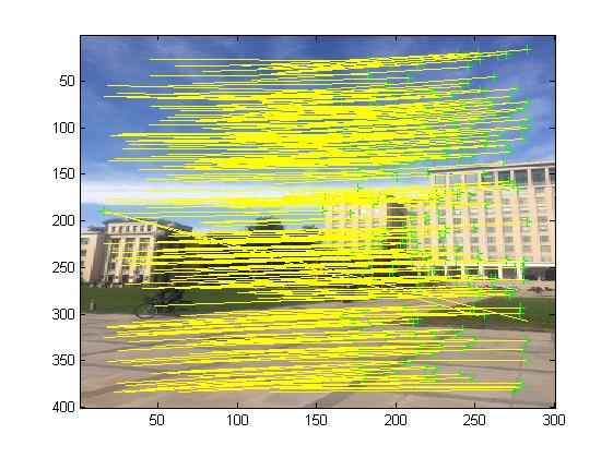
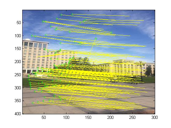
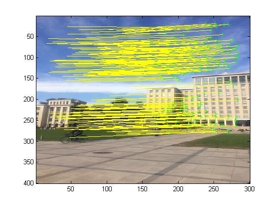
3, Operation results

4, matlab version and references

1 matlab version
2014a

2 references
[1] Cai Limei. MATLAB image processing theory, algorithm and example analysis [M]. Tsinghua University Press, 2020
[2] Yang Dan, Zhao Haibin, long Zhe. Detailed explanation of MATLAB image processing examples [M]. Tsinghua University Press, 2013
[3] Zhou pin. MATLAB image processing and graphical user interface design [M]. Tsinghua University Press, 2013
[4] Liu Chenglong. Proficient in MATLAB image processing [M]. Tsinghua University Press, 2015
[5] Hou Sizu, Chen Yu, Liu Yating. Research on image registration in UV imager based on mutual information [J]. Semiconductor optoelectronics. 2020,41 (04)