1, Introduction to differential evolution algorithm
1 Preface
Under the action of heredity, selection and variation, the survival of the fittest in nature continues to evolve and develop from low-level to high-level. It is noted that the evolutionary law of survival of the fittest can be modeled to form some optimization algorithms; Evolutionary algorithms developed in recent years have attracted extensive attention.
Differential Evolution (DE) is a new evolutionary computing technology [1]. It was proposed by storn et al. In 1995. Its initial idea was to solve the Chebyshev polynomial problem. Later, it was found that it is also an effective way to solve complex optimization problems
Efficient technology.
Differential evolution algorithm is an optimization algorithm based on swarm intelligence theory. It is an intelligent optimization search algorithm generated through the cooperation and competition among individuals in the group. However, compared with evolutionary computation, it retains the global search strategy based on population, and adopts the simple method of real number coding and difference based
Mutation operation and "one-to-one" competitive survival strategy reduce the complexity of evolutionary computing operation. At the same time, the unique memory ability of differential evolution algorithm enables it to dynamically track the current search situation to adjust its search strategy. It has strong global convergence ability and robustness,
Without the help of the characteristic information of the problem, it is suitable for solving some complex optimization problems that are difficult or even impossible to be solved by conventional mathematical programming methods [2-5]. Therefore, as an efficient parallel search algorithm, the theoretical and Application Research of differential evolution algorithm has important academic significance and engineering value.
At present, differential evolution algorithm has been applied in many fields, such as artificial neural network, electric power, mechanical design, robot, signal processing, biological information, economics, modern agriculture and operations research. However, although the differential evolution algorithm has been widely studied, it is relatively simple
For other evolutionary algorithms, their research results are quite scattered and lack of systematicness, especially in theory.
2 differential evolution algorithm theory
2.1 principle of differential evolution algorithm
Differential evolution algorithm is a random heuristic search algorithm, which is simple to use, has strong robustness and global optimization ability. It is a random search algorithm from the mathematical point of view and an adaptive iterative optimization process from the engineering point of view. In addition to good convergence, the differential evolution algorithm is very easy to understand and execute. It contains only a few control parameters, and the values of these parameters can remain unchanged in the whole iterative process. Differential evolution algorithm is a self-organizing minimization method, and users only need little input. Its key idea is different from the traditional evolutionary method: the traditional method uses the predetermined probability distribution function to determine the vector disturbance; The self-organizing program of differential evolution algorithm uses two randomly selected different vectors in the population to interfere with an existing vector, and each vector in the population has to interfere. Differential evolution algorithm uses a vector population, in which the random disturbance of population vector can be carried out independently, so it is parallel. If the cost of new vectors corresponding to function values is less than that of their predecessors, they will replace their predecessors.
Like other evolutionary algorithms, differential evolutionary algorithm also operates on the population of candidate solutions, but its population reproduction scheme is different from other evolutionary algorithms: it generates a new parameter vector by adding the weighted difference vector between two members of the population to the third member
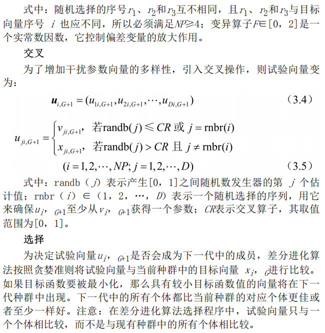
Called "variation"; Then, the parameters of the variation vector and other predetermined target vector parameters are mixed according to certain rules to produce the test quantity. This operation is called "crossover"; Finally, if the cost function of the test vector is lower than that of the objective vector, the test vector will replace the objective vector in the next generation. This operation is called "selection". All members of the population must do this once as target vectors so that the same number of competitors will appear in the next generation.
In the process of evolution, the optimal parameter vector of each generation is evaluated to record the minimization process. In this way, the method of generating new individuals by random deviation disturbance can obtain a very good convergence result and guide the search process to approach the global optimal solution [6-7].
2.2 characteristics of differential evolution algorithm
Differential evolution algorithm has been widely studied and successfully applied in just 20 years since it was proposed. The algorithm has the following characteristics:
(1) Simple structure and easy to use. Differential evolution algorithm mainly carries out genetic operation through differential mutation operator, which is easy to implement because it only involves the addition and subtraction of vectors; The algorithm adopts probability transfer rules and does not need deterministic rules. In addition, the differential evolution algorithm has few control parameters. The influence of these parameters on the performance of the algorithm has been studied, and some guiding suggestions have been obtained. Therefore, it is convenient for users to choose better parameter settings according to the problem.
(2) Superior performance. Differential evolution algorithm has good reliability, efficiency and robustness. For large space, nonlinear and non differentiable continuous problems, its solution efficiency is better than other evolutionary methods, and many scholars continue to improve differential evolution algorithm to continuously improve its performance.
(3) Adaptability. The differential mutation operator of differential evolution algorithm can be a fixed constant, or it can have the ability of adaptive mutation step size and search direction. It can be automatically adjusted according to different objective functions, so as to improve the search quality.
(4) Differential evolution algorithm has inherent parallelism, can cooperate in search, and has the ability to use individual local information and group global information to guide the algorithm to further search. Under the same accuracy requirements, differential evolution algorithm has faster convergence speed.
(5) The algorithm is general, and can directly operate the structure object, does not depend on the problem information, and there is no restriction on the objective function. Differential evolution algorithm is very simple and easy to program, especially for solving high-dimensional function optimization problems.
3 types of differential evolution algorithms
3.1 basic differential evolution algorithm
The operation procedure of basic differential evolution algorithm is as follows [8]:
(1) Initialization;
(2) Variation;
(3) Cross;
(4) Selection;
(5) Boundary condition treatment.
initialization
Differential evolution algorithm uses NP real valued parameter vectors with dimension D as each parameter vector
A population of one generation, each individual expressed as:
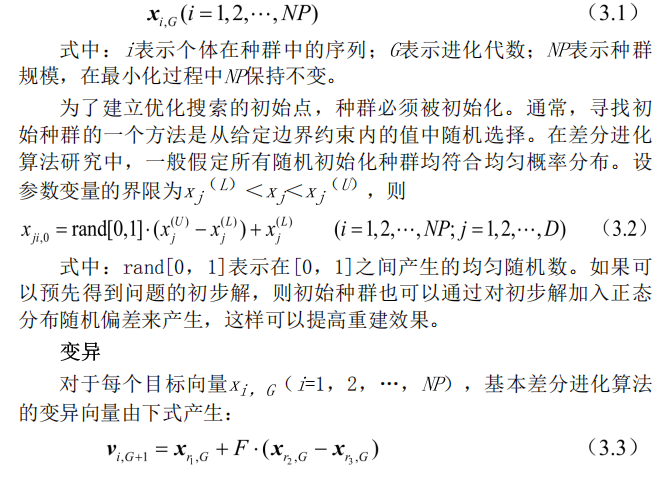
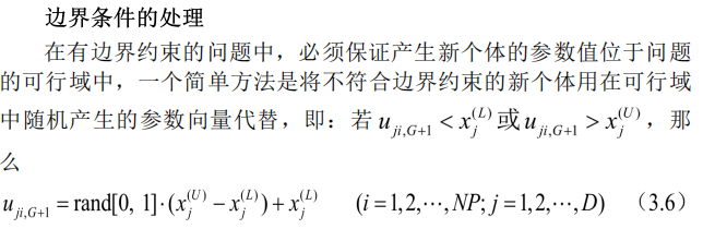
Another method is boundary absorption, that is, the individual value exceeding the boundary constraint is set to the adjacent boundary value.
3.2 other forms of differential evolution algorithm
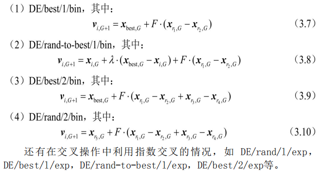
The above description is the most basic operation procedure of differential evolution algorithm. In practical application, several deformation forms of differential evolution algorithm are also developed, which are distinguished by the symbol DE/x/y/z, in which x defines that the currently mutated vector is "random" or "optimal"; y is the number of difference vectors used; z indicates the operation method of the crossover program. The cross operation described earlier is expressed as "bin". Using this representation, the basic differential evolution algorithm strategy can be described as DE/rand/1/bin.
There are other forms [5, such as:
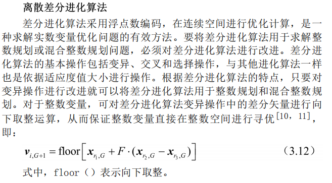
3.3 improved differential evolution algorithm
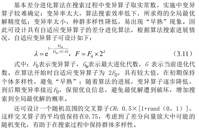
Adaptive differential evolution algorithm
As an efficient parallel optimization algorithm, differential evolution algorithm has developed rapidly, and there are many improved differential evolution algorithms. A differential evolution algorithm with adaptive operator is introduced below [9]
4 differential evolution algorithm flow
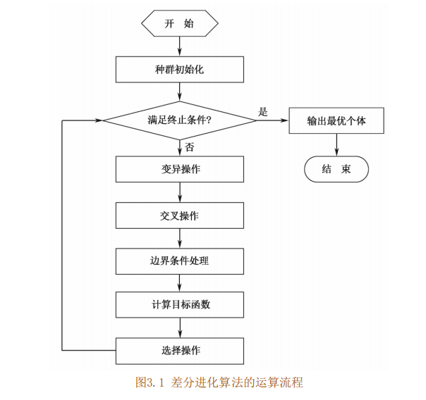
Differential evolution algorithm adopts real number coding, simple mutation operation based on difference and "one-to-one" competitive survival strategy. Its specific steps are as follows:
(1) Determine the control parameters and specific strategies of differential evolution algorithm. The control parameters of differential evolution algorithm include population number, mutation operator, crossover operator, maximum evolution algebra, termination condition and so on.
(2) The initial population is generated randomly, and the evolutionary algebra k=1.
(3) Evaluate the initial population, that is, calculate the objective function value of each individual in the initial population.
(4) Judge whether the termination condition is reached or the maximum evolutionary algebra is reached: if so, the evolution is terminated and the best individual at this time is used as the solution output; Otherwise, proceed to the next step.
(5) The mutation operation and crossover operation are carried out, and the boundary conditions are processed to obtain the temporary population.
(6) Evaluate the temporary population and calculate the objective function value of each individual in the temporary population.
(7) The individuals in the temporary population and the corresponding individuals in the original population are selected by "one pair -" to obtain the new population.
(8) Evolutionary algebra k=k+1, turn to step (4).
The operation flow of differential evolution algorithm is shown in Figure 3.1.
5 description of key parameters
The influence of control parameters on a global optimization algorithm is great, and there are some empirical rules for the selection of control variables in differential evolution algorithm.
Population number NP
Generally, the larger the population size AP, the more individuals, the better the diversity of the population, and the stronger the optimization ability, but it also increases the difficulty of calculation. Therefore, NP cannot be infinitely large. According to experience, the reasonable selection of population number NP is 5D~
Between 10D, NP ≥ 4 must be satisfied to ensure that the differential evolution algorithm has enough different mutation vectors.
Mutation operator F
The mutation operator FE[0,2] is a real constant factor, which determines the magnification of the deviation vector. If the mutation operator is small, the algorithm may be "premature". With the increase of / value, the ability to prevent the algorithm from falling into local optimization is enhanced, but when f > 1, it will become very difficult for the algorithm to quickly converge to the optimal value; This is because when the perturbation of the difference vector is greater than the distance between two individuals, the convergence of the population will become very poor. The current research shows that the values of F less than 0.4 and greater than 1 are only occasionally effective, and / = 0.5 is usually a good initial choice. If species
If the group converges prematurely, then F or NP should increase.
Crossover operator CR
The crossover operator CR is a real number in the range of [0,1], which controls the probability that a test vector parameter comes from the randomly selected mutation vector rather than the original vector. The greater the crossover operator CK, the greater the possibility of crossover. A better choice for CR is 0.1, but
Larger CK usually accelerates convergence. To see if it is possible to obtain a fast solution, try CR=0.9 or CF=1.0
Maximum evolutionary algebra G
The maximum evolution algebra 6 is a parameter representing the end condition of the differential evolution algorithm, which means that the differential evolution algorithm stops running after running to the specified evolution algebra, and outputs the best individual in the current population as the optimal solution of the problem. Generally, 6 is taken as 100 ~ 500.
Termination conditions
In addition to the maximum evolution algebra as the termination condition of differential evolution algorithm, other criteria can be added. Generally, when the value of the objective function is less than the threshold, the program terminates, and the threshold is often 10-6. Among the above parameters, F and CR, like NP, are constants in the search process. Generally, F and CR affect the convergence speed and robustness of the search process. Their optimization values depend not only on the characteristics of the objective function, but also on NP. Generally, after some tests on different values, the appropriate values of F, CR and NP can be found by using the test and result errors.
2, Complete source code
function [bestc,bestg,test_pre]=my_HGWO_SVR(para,input_train,output_train,input_test,output_test)
% Parameter vector parameters [n,N_iteration,beta_min,beta_max,pCR]
% n Is the population size, N_iteration Is the number of iterations
% beta_min Lower bound of scaling factor Lower Bound of Scaling Factor
% beta_max=0.8; % Upper bound of scaling factor Upper Bound of Scaling Factor
% pCR Crossover probability Crossover Probability
% The input data is required to be a column vector (matrix)
%% data normalization
[input_train,rule1]=mapminmax(input_train');
[output_train,rule2]=mapminmax(output_train');
input_test=mapminmax('apply',input_test',rule1);
output_test=mapminmax('apply',output_test',rule2);
input_train=input_train';
output_train=output_train';
input_test=input_test';
output_test=output_test';
%% Using differential evolution-Gray wolf optimization hybrid algorithm( DE_GWO)Choose the best SVR parameter
nPop=para(1); % Population size Population Size
MaxIt=para(2); % Maximum number of iterations Maximum Number of Iterations
nVar=2; % Independent variable dimension, two parameters need to be optimized in this example c and g Number of Decision Variables
VarSize=[1,nVar]; % Decision variable matrix size Decision Variables Matrix Size
beta_min=para(3); % Lower bound of scaling factor Lower Bound of Scaling Factor
beta_max=para(4); % Upper bound of scaling factor Upper Bound of Scaling Factor
pCR=para(5); % Crossover probability Crossover Probability
lb=[0.01,0.01]; % Lower bound of parameter value
ub=[100,100]; % Upper bound of parameter value
%% initialization
% Parent population initialization
parent_Position=init_individual(lb,ub,nVar,nPop); % Random initialization position
parent_Val=zeros(nPop,1); % Objective function value
for i=1:nPop % Traverse each individual
parent_Val(i)=fobj(parent_Position(i,:),input_train,output_train,input_test,output_test); % Calculate individual objective function value
end
% Mutation population initialization
mutant_Position=init_individual(lb,ub,nVar,nPop); % Random initialization position
mutant_Val=zeros(nPop,1); % Objective function value
for i=1:nPop % Traverse each individual
mutant_Val(i)=fobj(mutant_Position(i,:),input_train,output_train,input_test,output_test); % Calculate individual objective function value
end
% Progeny population initialization
child_Position=init_individual(lb,ub,nVar,nPop); % Random initialization position
child_Val=zeros(nPop,1); % Objective function value
for i=1:nPop % Traverse each individual
child_Val(i)=fobj(child_Position(i,:),input_train,output_train,input_test,output_test); % Calculate individual objective function value
end
%% Determine the parent population Alpha,Beta,Delta wolf
[~,sort_index]=sort(parent_Val); % Ranking of objective function values of parent population
parent_Alpha_Position=parent_Position(sort_index(1),:); % Determine parent Alpha wolf
parent_Alpha_Val=parent_Val(sort_index(1)); % Parent generation Alpha Wolf objective function value
parent_Beta_Position=parent_Position(sort_index(2),:); % Determine parent Beta wolf
parent_Delta_Position=parent_Position(sort_index(3),:); % Determine parent Delta wolf
%% Iteration start
BestCost=zeros(1,MaxIt);
BestCost(1)=parent_Alpha_Val;
for it=1:MaxIt
a=2-it*((2)/MaxIt); % For each iteration, calculate the corresponding a Value, a decreases linearly fron 2 to 0
% Update parent individual location
for par=1:nPop % Traverse parent individual
for var=1:nVar % Traverse each dimension
% Alpha wolf Hunting
r1=rand(); % r1 is a random number in [0,1]
r2=rand(); % r2 is a random number in [0,1]
A1=2*a*r1-a; % Calculation coefficient A
C1=2*r2; % Calculation coefficient C
D_alpha=abs(C1*parent_Alpha_Position(var)-parent_Position(par,var));
X1=parent_Alpha_Position(var)-A1*D_alpha;
% Beta wolf Hunting
r1=rand();
r2=rand();
A2=2*a*r1-a; % Calculation coefficient A
C2=2*r2; % Calculation coefficient C
D_beta=abs(C2*parent_Beta_Position(var)-parent_Position(par,var));
X2=parent_Beta_Position(var)-A2*D_beta;
% Delta wolf Hunting
r1=rand();
r2=rand();
A3=2*a*r1-a; % Calculation coefficient A
C3=2*r2; % Calculation coefficient C
D_delta=abs(C3*parent_Delta_Position(var)-parent_Position(par,var));
X3=parent_Delta_Position(var)-A3*D_delta;
% Location update to prevent cross-border
X=(X1+X2+X3)/3;
X=max(X,lb(var));
X=min(X,ub(var));
parent_Position(par,var)=X;
end
parent_Val(par)=fobj(parent_Position(par,:),input_train,output_train,input_test,output_test); % Calculate individual objective function value
end
% Produce variant (intermediate) population
for mut=1:nPop
A=randperm(nPop); % Individual order is rearranged randomly
A(A==i)=[]; % The position of the current individual is vacated (the current individual does not participate in the generation of variant intermediates)
a=A(1);
b=A(2);
c=A(3);
beta=unifrnd(beta_min,beta_max,VarSize); % Randomly generated scaling factor
y=parent_Position(a)+beta.*(parent_Position(b)-parent_Position(c)); % Produce intermediate
% Prevent intermediate from crossing the boundary
y=max(y,lb);
end
% Generation of progeny population, cross operation Crossover
for child=1:nPop
x=parent_Position(child,:);
y=mutant_Position(child,:);
z=zeros(size(x)); % Initialize a new individual
j0=randi([1,numel(x)]); % Generate a pseudo-random number, that is, select the dimension number to be exchanged???
for var=1:numel(x) % Traverse each dimension
if var==j0 || rand<=pCR % If the current dimension is the dimension to be exchanged or the random probability is less than the crossover probability
z(var)=y(var); % The current dimension value of the new individual is equal to the corresponding dimension value of the intermediate
else
z(var)=x(var); % The current dimension value of the new individual is equal to the corresponding dimension value of the current individual
end
end
child_Position(child,:)=z; % New individuals are obtained after cross operation
child_Val(child)=fobj(z,input_train,output_train,input_test,output_test); % New individual objective function value
end
% Parent population renewal
for par=1:nPop
if child_Val(par)<parent_Val(par) % If the offspring is better than the parent
parent_Val(par)=child_Val(par); % Update parent individual
end
end
% Determine the parent population Alpha,Beta,Delta wolf
[~,sort_index]=sort(parent_Val); % Ranking of objective function values of parent population
parent_Alpha_Position=parent_Position(sort_index(1),:); % Determine parent Alpha wolf
parent_Alpha_Val=parent_Val(sort_index(1)); % Parent generation Alpha Wolf objective function value
parent_Beta_Position=parent_Position(sort_index(2),:); % Determine parent Beta wolf
parent_Delta_Position=parent_Position(sort_index(3),:); % Determine parent Delta wolf
BestCost(it)=parent_Alpha_Val;
end
bestc=parent_Alpha_Position(1,1);
bestg=parent_Alpha_Position(1,2);
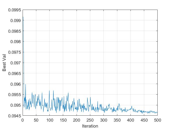
%% Graphical optimization process
plot(BestCost);
xlabel('Iteration');
ylabel('Best Val');
grid on;
%% Regression prediction was used to analyze the best parameters SVM Network training
%% SVM Network regression prediction
[output_test_pre,~]=svmpredict(output_test,input_test,model_cs_svr); % SVM Model prediction and its accuracy
test_pre=mapminmax('reverse',output_test_pre',rule2);
test_pre = test_pre';
%% SVR_fitness -- objective function
function fitness=fobj(cv,input_train,output_train,input_test,output_test)
% cv Is the transverse quantity with length 2, i.e SVR Medium parameter c and v Value of
cmd = ['-s 3 -t 2',' -c ',num2str(cv(1)),' -g ',num2str(cv(2))];
model=svmtrain(output_train,input_train,cmd); % SVM model training
[~,fitness]=svmpredict(output_test,input_test,model); % SVM Model prediction and its accuracy
fitness=fitness(2); % Average mean square error MSE As the objective function value of optimization
function x=init_individual(xlb,xub,dim,sizepop)
% Parameter initialization function
% lb: Parameter lower bound, row vector
% ub: Parameter upper bound, row vector
% dim: Parameter dimension
% sizepop Population size
% x: return sizepop*size(lb,2)Parameter matrix of
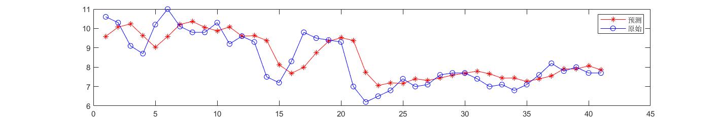
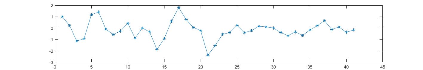
3, Operation results
4, matlab version and references
1 matlab version
2014a
2 references
Intelligent optimization algorithm and its MATLAB example (2nd Edition), written by baozi Yang Yu Ji Zhou Yang Shan, electronic industry press