1, Introduction to UAV
0 Introduction
With the development of modern technology, there are more and more types of aircraft, and their applications are becoming more and more specific and perfect, such as Dajiang PS-X625 UAV specially used for plant protection, Baoji Xingyi aviation technology X8 UAV used for street view shooting and monitoring patrol, and white shark MIX underwater UAV used for underwater rescue, The performance of aircraft is mainly determined by the internal flight control system and external path planning. As far as the path problem is concerned, only relying on the remote controller in the operator's hand to control the UAV to perform the corresponding work during the specific implementation of the task may put forward high requirements for the operator's psychology and technology. In order to avoid personal operation errors and the risk of aircraft damage, one way to solve the problem is to plan the flight path of the aircraft.
These changes, such as the measurement accuracy of aircraft, the reasonable planning of track path, the stability and safety of aircraft, have higher and higher requirements for the integrated control system of aircraft. UAV route planning is to design the optimal route to ensure that UAV can complete a specific flight mission and avoid various obstacles and threat areas in the process of completing the mission.
1 common track planning algorithms
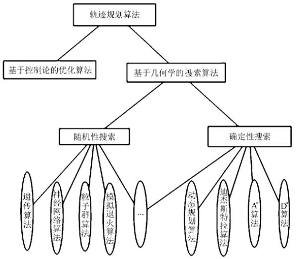
Figure 1 common path planning algorithms
This paper mainly studies the path planning of UAV in the cruise phase. Assuming that the UAV maintains the same altitude and speed in flight, the path planning becomes A two-dimensional plane planning problem. In the track planning algorithm, A algorithm is simple and easy to implement. Based on the improved A algorithm, A new and easy to understand UAV track planning method based on the improved A algorithm is proposed. The traditional A algorithm rasterizes the planning area, and the node expansion is limited to the intersection of grid lines. There are often two motion directions with A certain angle between the intersection and intersection of grid lines. Infinitely enlarge and refine the two paths with angles, and then use the corresponding path planning points on the two segments as the tangent points to find the center of the corresponding inscribed circle, and then make an arc, calculate the center angle of the arc between the corresponding two tangent points, and calculate the length of the arc according to the following formula

Where: R - radius of inscribed circle;
α——— The center angle corresponding to the arc between tangent points.
2, Introduction to particle swarm optimization
1 Introduction
The group behavior of birds and fish in nature has always been the research interest of scientists. Biologist Craig Reynolds proposed a very influential bird swarm aggregation model in 1987. In his simulation, each individual follows: avoid collision with neighboring individuals: match the speed of neighboring individuals; Fly to the center of the flock, and the whole flock flies to the target. In the simulation, only the above three simple rules can be used to closely simulate the phenomenon of birds flying. In 1990, biologist Frank Heppner also proposed a bird model. The difference is that birds are attracted to fly to their habitat. In the simulation, at the beginning, each bird has no specific flight target, but uses simple rules to determine its flight direction and speed. When a bird flies to the habitat, the birds around it will fly to the habitat, and finally the whole flock will land in the habitat.
In 1995, American social psychologist James Kennedy and electrical engineer Russell Eberhart jointly proposed particle swarm optimization (PSO), which was inspired by the research results of modeling and Simulation of bird group behavior. Their models and simulation algorithms mainly modify Frank Heppner's model to make the particles fly to the solution space and land at the optimal solution. Once particle swarm optimization algorithm was proposed, because its algorithm is simple and easy to implement, it immediately attracted extensive attention of scholars in the field of evolutionary computing and formed a research hotspot. Swarm intelligence published by J.Kennedy and R.Eberhart in 2001 further expanded the influence of swarm intelligence [], and then a large number of research reports and research results on particle swarm optimization algorithm emerged, which set off a research upsurge at home and abroad [2-7].
Particle swarm optimization algorithm comes from the regularity of bird group activities, and then uses swarm intelligence to establish a simplified model. It simulates the foraging behavior of birds, compares the search space for solving the problem to the flight space of birds, and abstracts each bird into a particle without mass and volume
The process of finding the optimal solution of the problem is regarded as the process of birds looking for food, and then the complex optimization problem is solved. Like other evolutionary algorithms, particle swarm optimization algorithm is also based on the concepts of "population" and "evolution"
Cooperation and competition to realize the search of optimal solution in complex space. At the same time, unlike other evolutionary algorithms, it performs evolutionary operator operations such as crossover, mutation and selection on individuals. Instead, it regards individuals in the population as particles without mass and volume in the l-dimensional search space. Each particle moves in the solution space at a certain speed and gathers to its own historical best position P best and neighborhood historical best position g best, Realize the evolution of candidate solutions. Particle swarm optimization algorithm has a good biological and social background and is easy to understand. Due to few parameters and easy to implement, it has strong global search ability for nonlinear and multimodal problems. It has attracted extensive attention in scientific research and engineering practice. At present, the algorithm has been widely used in function optimization, neural network training, pattern classification, fuzzy control and other fields.
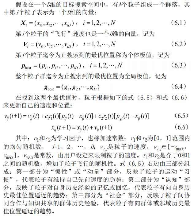
2 particle swarm optimization theory
2.1 description of particle swarm optimization algorithm
In the process of bird predation, members of the flock can obtain the discovery and flight experience of other members through information exchange and sharing among individuals. Under the condition that food sources are sporadically distributed and unpredictable, the advantages brought by this cooperation mechanism are decisive, far greater than the impact on food
Disadvantages caused by competition. Inspired by the predation behavior of birds, particle swarm optimization algorithm simulates this behavior. The search space of the optimization problem is compared with the flight space of birds. Each bird is abstracted as a particle. The particle has no mass and volume to represent a feasible solution of the problem. The optimal solution to be searched for in the optimization problem is equivalent to the food source sought by birds. Particle swarm optimization algorithm formulates simple behavior rules for each particle similar to bird motion, so that the motion of the whole particle swarm shows similar characteristics to bird predation, so it can solve complex optimization problems.
The information sharing mechanism of particle swarm optimization algorithm can be interpreted as a symbiotic and cooperative behavior, that is, each particle is constantly searching, and its search behavior is affected by other individuals in the group to varying degrees [8]. At the same time, these particles also have the memory of the best position they experience
Memory ability, that is, its search behavior is not only influenced by other individuals, but also guided by its own experience. Based on the unique search mechanism, particle swarm optimization algorithm first generates the initial population, that is, randomly initializes the velocity and position of particles in the feasible solution space and velocity space, in which the position of particles is used to represent the feasible solution of the problem, and then solves the optimization problem through the cooperation and competition of individual particles among populations.
2.2 particle swarm optimization modeling
Particle swarm optimization algorithm comes from the study of bird predation behavior: a group of birds randomly search for food in the area. All birds know how far their current position is from the food, so the simplest and effective strategy is to search the surrounding area of the bird nearest to the food. Particle swarm optimization
This model is used to get enlightenment and applied to solve optimization problems. In particle swarm optimization, the potential solution of each optimization problem is a bird in the search space, which is called particle. All particles have a fitness value determined by the optimized function, and each particle has a speed to determine their flying direction and distance. Then, the particles follow the current optimal particle to search in the solution space [9].
Firstly, particle swarm optimization algorithm initializes particle swarm randomly in a given solution space, and the number of variables of the problem to be optimized determines the dimension of the solution space. Each particle has an initial position and initial velocity, and then it is optimized by iteration. In each iteration, each particle updates its spatial position and flight speed in the solution space by tracking two "extreme values": one extreme value is the optimal solution particle found by a single particle in the iteration process, which is called individual extreme value; the other extreme value is the optimal solution particle found by all particles in the population in the iteration process, This particle is a global extremum. The above method is called global particle swarm optimization. If you do not use all particles in the population and only use a part of them as the neighbor particles of the particle, the extreme value in all neighbor particles is the local extreme value. This method is called local particle swarm optimization algorithm.
2.3 characteristics of particle swarm optimization algorithm
Particle swarm optimization is essentially a random search algorithm. It is a new intelligent optimization technology. The algorithm can converge to the global optimal solution with high probability. Practice shows that it is suitable for optimization in dynamic and multi-objective optimization environment. Compared with traditional optimization algorithms, it has faster calculation speed
Computing speed and better global search ability.
(1) Particle swarm optimization algorithm is an optimization algorithm based on swarm intelligence theory. It guides the optimization search through the swarm intelligence generated by the cooperation and competition among particles in the swarm. Compared with other algorithms, particle swarm optimization is an efficient parallel search algorithm.
(2) Both particle swarm optimization algorithm and genetic algorithm initialize the population randomly, and use fitness to evaluate the quality of individuals and carry out a certain random search. However, particle swarm optimization algorithm determines the search according to its own speed, without the crossover and mutation of genetic algorithm. Compared with evolutionary algorithm, particle swarm optimization algorithm retains the global search strategy based on population, but its speed displacement model is simple to operate and avoids complex genetic operations.
(3) Because each particle still maintains its individual extreme value at the end of the algorithm, that is, particle swarm optimization algorithm can not only find the optimal solution of the problem, but also get some better suboptimal solutions. Therefore, applying particle swarm optimization algorithm to scheduling and decision-making problems can give a variety of meaningful schemes.
(4) The unique memory of particle swarm optimization makes it possible to dynamically track the current search situation and adjust its search strategy. In addition, particle swarm optimization algorithm is not sensitive to the size of population. Even when the number of population decreases, the performance degradation is not great.
3 types of particle swarm optimization
3.1 basic particle swarm optimization
3.2 standard particle swarm optimization algorithm
Two concepts often used in the study of particle swarm optimization are introduced: one is "exploration", which means that particles leave the original search track to a certain extent and search in a new direction, which reflects the ability to explore unknown areas, similar to global search; The second is "development", which means that particles continue to search in a finer step on the original search track to a certain extent, mainly referring to further searching the areas searched in the exploration process. Exploration is to deviate from the original optimization trajectory to find a better solution. Exploration ability is the global search ability of an algorithm. Development is to use a good solution and continue the original optimization trajectory to search for a better solution. It is the local search ability of the algorithm. How to determine the proportion of local search ability and global search ability is very important for the solution process of a problem. In 1998, Shi Yuhui et al. Proposed an improved particle swarm optimization algorithm with inertia weight [10]. Because the algorithm can ensure good convergence effect, it is defaulted to the standard particle swarm optimization algorithm. Its evolution process is:
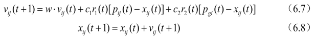
In equation (6.7), the first part represents the previous velocity of the particle, which is used to ensure the global convergence performance of the algorithm; The second and third parts make the algorithm have local convergence ability. It can be seen that the inertia weight W in equation (6.7) represents the extent to which the original speed is retained: W
Larger, the global convergence ability is strong and the local convergence ability is weak; If w is small, the local convergence ability is strong and the global convergence ability is weak.
When w=1, equation (6.7) is exactly the same as equation (6.5), indicating that the particle swarm optimization algorithm with inertia weight is an extension of the basic particle swarm optimization algorithm. The experimental results show that when w is between 0.8 and 1.2, PSO has faster convergence speed; When w > 1.2, the algorithm is easy to fall into local extremum.
In addition, w can be dynamically adjusted in the search process: at the beginning of the algorithm, w can be given a large positive value. With the progress of the search, w can be gradually reduced linearly, which can ensure that each particle can explore in the global range with a large speed step at the beginning of the algorithm
Good area is measured; In the later stage of the search, the smaller W value ensures that the particles can do a fine search around the extreme point, so that the algorithm has a greater probability of converging to the global optimal solution. Adjusting w can balance the ability of global search and local search. At present, the more dynamic inertia weight value is the linear decreasing weight strategy proposed by Shi, and its expression is as follows:
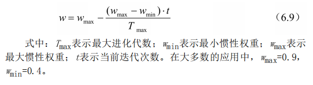
3.3 compression factor particle swarm optimization algorithm
Clerc et al. Proposed using constraint factors to control the final convergence of system behavior [11]. This method can effectively search different regions and obtain high-quality solutions. The speed update formula of compression factor method is:
The experimental results show that compared with the particle swarm optimization algorithm using inertia weight, the
Particle swarm optimization algorithm with constraint factor has faster convergence speed.
3.4 discrete particle swarm optimization
The basic particle swarm optimization algorithm is a powerful tool to search the extreme value of function in continuous domain. After the basic particle swarm optimization algorithm, Kennedy and Eberhart proposed a discrete binary version of particle swarm optimization algorithm [12]. In this discrete particle swarm optimization method, the discrete problem space is mapped to the continuous particle motion space, and the particle swarm optimization algorithm is modified appropriately to solve it. In the calculation, the speed position update operation rules of the classical particle swarm optimization algorithm are still retained. The values and changes of particles in state space are limited to 0 and 1, and each dimension vi y of velocity represents the possibility that each bit xi of position is taken as 1. Therefore, the vij update formula in continuous particle swarm optimization remains unchanged, but P best and: best only take values in [0,1]. The position update equation is expressed as follows:
4 particle swarm optimization process
Based on the concepts of "population" and "evolution", particle swarm optimization algorithm realizes the search of optimal solution in complex space through individual cooperation and competition [13]. Its process is as follows:
(1) Initializing particle swarm, including population size N and position x of each particle; And speed Vio
(2) Calculate the fitness value of each particle fit[i].
(3) For each particle, compare its fitness value fit [gate with the individual extreme value P best(i). If fit[i] < P best(i), replace P best(i) with fit[i].
(4) For each particle, its fitness value fit[i] is compared with the global extremum g best. If fit[i] < 8 best, replace g best with fit[i].
(5) Iteratively update the particle velocity v; And location xj.
(6) Carry out boundary condition treatment.
(7) Judge whether the termination conditions of the algorithm are met: if so, end the algorithm and output the optimization results; Otherwise, return to step (2).
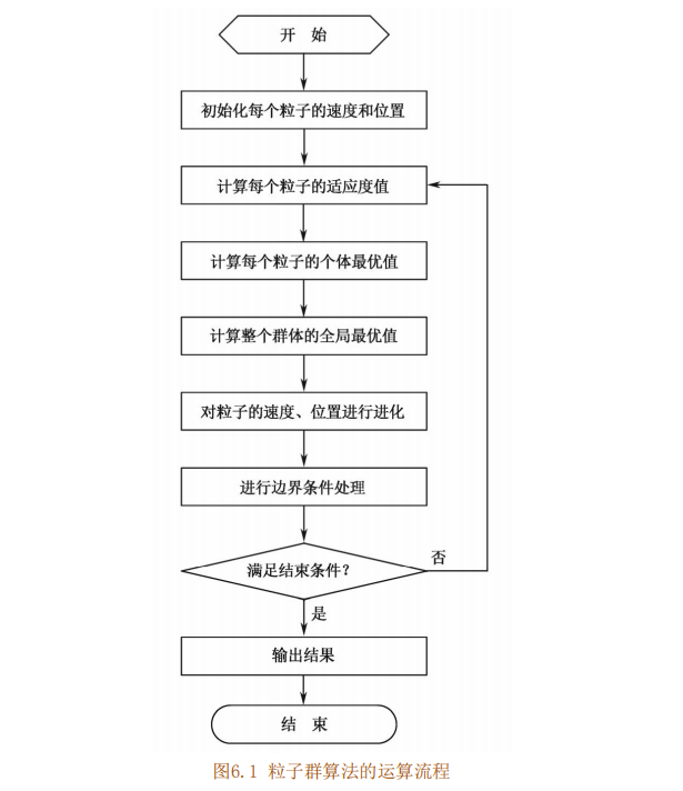
The operation flow of particle swarm optimization algorithm is shown in Figure 6.1.
5 description of key parameters
In particle swarm optimization algorithm, the selection of control parameters can affect the performance and efficiency of the algorithm; How to select appropriate control parameters to optimize the performance of the algorithm is a complex optimization problem. In practical optimization problems, the control parameters are usually selected according to the user's experience.
The control parameters of particle swarm optimization algorithm mainly include: particle population size N, inertia weight w, acceleration coefficients c and c, maximum speed Via x, stop criterion, setting of neighborhood structure, boundary condition processing strategy, etc. [14],
Particle population size N
The selection of particle population size depends on the specific problem, but the number of particles is generally set to 20 ~ 50. For most problems, 10 particles can achieve good results: however, for difficult problems or specific types of problems, the number of particles can be taken as 100 or 100
200. In addition, the larger the number of particles, the larger the search space of the algorithm, and it is easier to find the global optimal solution; Of course, the longer the algorithm runs.
Inertia weight w
Inertia weight w is a very important control parameter in standard particle swarm optimization algorithm, which can be used to control the development and exploration ability of the algorithm. The size of the inertia weight indicates how much is inherited from the particle's current velocity. When the inertia weight value is large, the global optimization ability is strong and the local optimization ability is strong
Weak: when the inertia weight value is small, the global optimization ability is weak and the local optimization ability is strong. The choice of inertia weight usually has fixed weight and time-varying weight. Fixed weight is to select a constant as the inertia weight value, which remains unchanged in the process of evolution. Generally, the value is
[0.8, 1.2]: time-varying weight is to set a change interval and gradually reduce the inertia weight in a certain way in the process of evolution. The selection of time-varying weight includes variation range and decline rate. Fixed inertia weight can make particles maintain the same exploration and development ability, while time-varying weight can make particles have different exploration and development ability in different stages of evolution.
Acceleration constants c1 and c2
The acceleration constants c and c 2 adjust the maximum step length in the direction of P best and g best respectively. They determine the influence of particle individual experience and group experience on particle trajectory respectively, and reflect the information exchange between particle swarm. If cr=c2=0, the particles will fly to the boundary at their current flight speed. At this time, particles can only search a limited area, so it is difficult to find the optimal solution. If q=0, it is a "social" model. Particles lack cognitive ability and only have group experience. Its convergence speed is fast, but it is easy to fall into local optimization; If oy=0, it is the "cognitive" module
Type, there is no social shared information, and there is no information interaction between individuals, so the probability of finding the optimal solution is small. A group with scale D is equivalent to running N particles. Therefore, generally set c1=C2, and generally take c1=cg=1.5. In this way, individual experience and group experience have the same important influence, making the final optimal solution more accurate.
Maximum particle velocity vmax
The speed of particles has a maximum speed limit value vd max on each dimension of space, which is used to clamp the speed of particles and control the speed within the range [- Vimax, + va max], which determines the strength of problem space search. This value is generally set by the user. Vmax is a very important parameter. If the value is too large, the particles may fly over the excellent region; if the value is too small, the particles may not be able to fully detect the region outside the local optimal region. They may fall into the local optimum and cannot move far enough to jump out of the local optimum and reach a better position in space. The researchers pointed out that setting Vmax and adjusting inertia weight are equivalent, so! max is generally used to set the initialization of the population, that is, Vmax is set as the variation range of each dimensional variable, instead of carefully selecting and adjusting the maximum speed.
Stop criteria
The maximum number of iterations, calculation accuracy or the maximum number of stagnant steps of the optimal solution ▲ t (or acceptable satisfactory solution) are usually regarded as the stop criterion, that is, the termination condition of the algorithm. According to the specific optimization problem, the setting of stop criterion needs to take into account the solution time, optimization quality and efficiency of the algorithm
Search efficiency and other performance.
Setting of neighborhood structure
The global version of particle swarm optimization takes the whole population as the neighborhood of particles, which has the advantage of fast convergence, but sometimes the algorithm will fall into local optimization. The local version of particle swarm optimization takes the individuals with similar positions as the neighborhood of particles, which converges slowly and is not easy to fall into local optimization
Value. In practical application, the global particle swarm optimization algorithm can be used to find the direction of the optimal solution, that is, the approximate results can be obtained, and then the local particle swarm optimization algorithm can be used to carry out fine search near the best point.
Boundary condition treatment
When the position or velocity of a one-dimensional or dry dimension exceeds the set value, the boundary condition processing strategy can limit the position of particles to the feasible search space, which can not only avoid the expansion and divergence of the population, but also avoid the blind search of particles in a large range, so as to improve the search efficiency.
There are many specific methods. For example, by setting the maximum position limit Xmax and the maximum speed limit Vmax, when the maximum position or maximum speed is exceeded, a numerical value is randomly generated within the range to replace it, or set it to the maximum value, that is, boundary absorption.
3, Partial source code
%% PSO 3D path planning
clc,clear , close all
feature jit off
%% Basic parameters of model
% Load terrain matrix
filename = 'TestData1.xlsx' ;
model.x_data = xlsread( filename , 'Xi') ;
model.y_data = xlsread(filename, 'Yi') ;
model.z_data = xlsread( filename , 'Zi') ;
model.x_grid = model.x_data(1,:) ;
model.y_grid =model.y_data(:, 1) ;
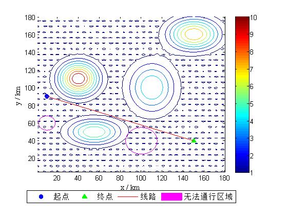
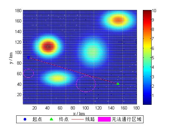
model.xs = 10 ; %Starting point related information
model.ys = 90 ;
model.zs = interp2( model.x_data , model.y_data, model.z_data , ...
model.xs , model.ys ,'linear' ) ; % The height is obtained by interpolation
model.xt = 150 ; % End point related information
model.yt = 40 ;
model.zt = interp2( model.x_data , model.y_data, model.z_data , ...
model.xt , model.yt , 'linear'); % The height is obtained by interpolation
model.n= 5 ; % Coarse navigation point settings
model.nn= 80 ; % Total number of navigation points obtained by interpolation
model.Safeh = 0.01 ; % Minimum flight altitude with obstacles
% Navigation point boundary value
model.xmin= min( model.x_data( : ) ) ;
model.xmax= max ( model.x_data( : ) ) ;
model.ymin= min( model.y_data( : ) ) ;
model.ymax= max( model.y_data( : ) ) ;
model.zmin= min( model.z_data( : ) ) ;
model.zmax =model.zmin + (1+ 0.1)*( max( model.z_data(:) )-model.zmin ) ;
% Other parameters of the model
model.nVar = 3*model.n ; % Coding length
model.pf = 10^7 ; % Penalty coefficient
% Obstacle location coordinates and radius
model.Barrier = [10,60 , 8 ;
100, 40, 15 ] ;
model.Num_Barrier = size(model.Barrier , 1 ); % Number of obstacles
model.weight1 = 0.5; % Weight 1 flight path length weight
model.weight2 = 0.3; % Weight 2 flight altitude related weight
model.weight3 = 0.2; % Weight 3 Jsmooth Index weight
%% Algorithm parameter setting
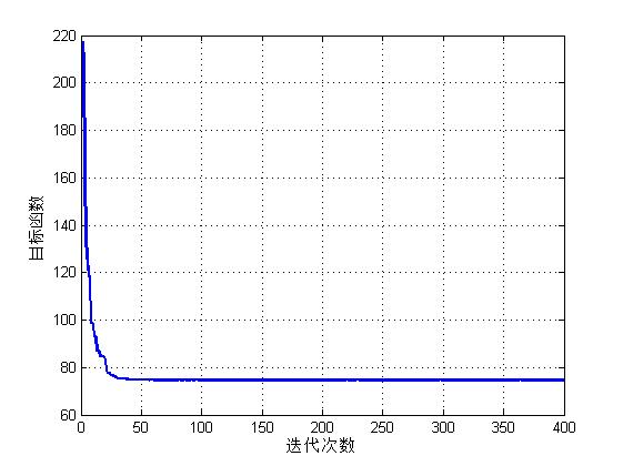
param.MaxIt = 400; % Number of iterations
param.nPop= 20; % Population number
param.w=1; % weight
param.wdamp=0.99; % Degradation rate
param.c1=1.5; % Personal Learning Coefficient
param.c2=2 ; % Global Learning Coefficient
% Partial parameters of local search
param.MaxSubIt= 0; % Maximum Number of Sub-iterations ( Number of internal loop iterations )
param.T = 25; %
param.alpha1=0.99; % Temp. Reduction Rate
param.ShowIteration = 400; % How many iterations does the graph display
%% Run algorithm
CostFunction=@(x) MyCost(x,model); % Set objective function
[ GlobalBest , BestCost ] = pso( param , model , CostFunction ) ;
function [ GlobalBest , BestCost ] = pso( param , model , CostFunction )
%% PSO Algorithmic robot path planning (Fusion simulated annealing local search )
% Problem Definition
% CostFunction=@(x) MyCost(x,model); % Objective function value (line)
nVar = model.nVar ; % Number of nodes
VarSize=[1 nVar]; % Decision variable dimension
VarMin = 0 ; % Lower order of independent variable value
VarMax= 1 ;% Higher order of independent variable value
%% PSO Parameters
MaxIt= param.MaxIt ; % Number of iterations
nPop= param.nPop ; % Population number
w= param.w ; % weight
wdamp=param.wdamp ; % Degradation rate
c1= param.c1 ; % Personal Learning Coefficient
c2= param.c2 ; % Global Learning Coefficient
VelMax = 0.1* (VarMax - VarMin ); % X Maximum speed
VelMin = -VelMax ; % X Minimum speed
% Simulated annealing parameters
MaxSubIt= param.MaxSubIt ; % Maximum Number of Sub-iterations
T = param.T ; %
alpha1= param.alpha1; % Temp. Reduction Rate
%% initialization
rand('seed', sum(clock));
% Create Empty Particle Structure
empty_particle.Position=[];
empty_particle.Velocity=[];
empty_particle.Cost=[];
empty_particle.Sol=[];
empty_particle.Best.Position=[];
empty_particle.Best.Cost=[];
empty_particle.Best.Sol=[];
% Initialize Global Best
GlobalBest.Cost=inf;
% Create Particles Matrix
particle=repmat(empty_particle,nPop,1);
% Initialization Loop
for i=1:nPop
% Initialize Position
particle(i).Position = unifrnd( VarMin , VarMax , VarSize ) ;
% Initialize Velocity
particle(i).Velocity = unifrnd( VelMin , VelMax , VarSize ) ;
% Evaluation
[particle(i).Cost, particle(i).Sol]=CostFunction(particle(i).Position);
% Update Personal Best
particle(i).Best.Position=particle(i).Position;
particle(i).Best.Cost=particle(i).Cost;
particle(i).Best.Sol=particle(i).Sol;
% Update Global Best
if particle(i).Best.Cost < GlobalBest.Cost
GlobalBest = particle(i).Best;
end
end
% Optimal solution record
BestCost=zeros(MaxIt,1);
%% PSO Main Loop
%%
for it=1:MaxIt
for i=1:nPop
% Update Velocity
particle(i).Velocity = w*particle(i).Velocity ...
+ c1*rand(VarSize).*(particle(i).Best.Position-particle(i).Position) ...
+ c2*rand(VarSize).*(GlobalBest.Position-particle(i).Position);
% Update Velocity Bounds
particle(i).Velocity = max(particle(i).Velocity,VelMin);
particle(i).Velocity = min(particle(i).Velocity,VelMax);
% Update Position
particle(i).Position = particle(i).Position + particle(i).Velocity ;
% Update Position Bounds
particle(i).Position = max(particle(i).Position,VarMin);
particle(i).Position = min(particle(i).Position,VarMax);
% Evaluation
[particle(i).Cost, particle(i).Sol]=CostFunction(particle(i).Position);
% Update Personal Best
if particle(i).Cost<particle(i).Best.Cost
particle(i).Best.Position=particle(i).Position;
particle(i).Best.Cost=particle(i).Cost;
particle(i).Best.Sol=particle(i).Sol;
% Update Global Best
if particle(i).Best.Cost<GlobalBest.Cost
GlobalBest=particle(i).Best;
end
end
end
%%
sol =GlobalBest ;
for subit=1:MaxSubIt
% Create and Evaluate New Solution
newsol.Position = Mutate( sol.Position ,VarMin,VarMax) ;
[ newsol.Cost , newsol.Sol ] =CostFunction( newsol.Position );
if newsol.Cost<= sol.Cost % If NEWSOL is better than SOL
sol = newsol;
else % If NEWSOL is NOT better than SOL
DELTA=(newsol.Cost-sol.Cost)/sol.Cost;
P= exp(-DELTA/T) ;
if rand<=P
sol= newsol ;
end
end
% Update Best Solution Ever Found
if sol.Cost<= GlobalBest.Cost
GlobalBest = sol ;
end
end
% Update Temp.
T=alpha1*T;
%%
% Update optimal solution
BestCost(it)=GlobalBest.Cost;
%Weight update
w=w*wdamp;
% Show Iteration Information
if GlobalBest.Sol.IsFeasible
Flag=' *';
else
Flag=[', Violation = ' num2str(GlobalBest.Sol.Violation)];
end
disp(['Iteration ' num2str(it) ': Best Cost = ' num2str(BestCost(it)) Flag]);
if ~mod( it, param.ShowIteration ) | isequal( it , MaxIt )
gcf = figure(1);
% Plot Solution
set(gcf, 'unit' ,'centimeters' ,'position',[5 2 25 15 ]);
GlobalBest.BestCost = BestCost(1:it) ;
GlobalBest.MaxIt = MaxIt ;
PlotSolution(GlobalBest ,model)
pause( 0.01 );
end
end
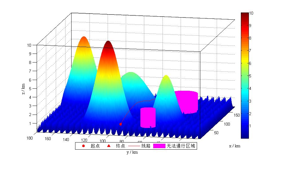
4, Operation results
5, matlab version and references
1 matlab version
2014a
2 references
[1] Steamed stuffed bun Yang, Yu Jizhou, Yang Shan Intelligent optimization algorithm and its MATLAB example (2nd Edition) [M]. Electronic Industry Press, 2016
[2] Zhang Yan, Wu Shuigen MATLAB optimization algorithm source code [M] Tsinghua University Press, 2017
[3] Wu Xi, Luo Jinbiao, Gu Xiaoqun, Zeng Qing Optimization algorithm of UAV 3D track planning based on Improved PSO [J] Journal of ordnance and equipment engineering 2021,42(08)
[4] Deng ye, Jiang Xiangju Four rotor UAV path planning algorithm based on improved artificial potential field method [J] Sensors and microsystems 2021,40(07)
[5] Ma Yunhong, Zhang Heng, Qi Lerong, he Jianliang 3D UAV path planning based on improved A * algorithm [J] Electro optic and control 2019,26(10)
[6] Jiao Yang Research on UAV 3D path planning based on improved ant colony algorithm [J] Ship electronic engineering 2019,39(03)