Introduction of template matching algorithm
1 Overview
Pattern recognition is to study the automatic processing and interpretation of patterns by solving mathematical models through computers. Among the various methods of pattern recognition, template matching is the easiest one, and its mathematical model is easy to establish. Digital image pattern recognition through template matching is helpful for us to understand the application of mathematical model in digital image.
2 template matching algorithm
2.1 similarity measure matching
The practical operation idea of template matching is very simple: take the known template and match an area of the same size as the original image. At the beginning, the upper left corner of the template coincides with the upper left corner of the image. Take an area of the same size in the template and the original image to compare, then translate to the next pixel, and still perform the same operation,... After all the positions are aligned, the object with the smallest difference is the object we are looking for.
The above description is the solution idea of matching by similarity measure method, and its operation in the computer is shown in Figure 2. Let the template t be superimposed on the search graph and translated, and the image under the search graph covered by the template is called the subgraph Si, J, I, J, which is the coordinate of the upper left corner pixel of this subgraph in the s graph, which is called the reference point. It can be seen from Figure 2 that the value range of I, j is: 1 < I, J < n - M + 1 Now we can compare the contents of T and Si, J. If the two are consistent, the difference between T and S is zero Therefore, the following formulas (1) and (2) can be used to measure the similarity between T and Si, J.
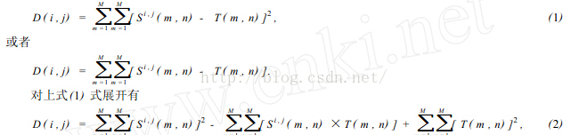

In equation (2), item 3 represents the total energy of the template, which is a constant independent of (I, J); The first item is the energy of the template covering subgraph, which changes slowly with the position of (I, J); The relationship between the subgraph and the template represented by item 2 changes with the change of (I, J). When T matches Si, J, this value is the largest. Therefore, the following correlation function (3) can be used as a similarity measure.
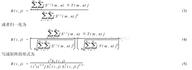
When the included angle between vector t and S1 is 0, that is, when S1 (I, J) = KT (k is a constant), there is R (I, J) = 1, otherwise R (I, J) < 1 Obviously, the larger R (I, J), the more similar the template T and Si, J. the point (I, J) is the matching point we are looking for.
2.2 sequential similarity detection algorithm
The calculation amount of matching by correlation method is very large, because the template needs to make correlation calculation at (n - M + 1) two reference positions. Except at the matching points, other points do useless work. Therefore, an algorithm called sequential similarity detection algorithm (SSDA) is proposed. Its key points are as follows:
In the digital image, the SSDA method uses formula (6) to calculate the non similarity m (I, J) of image f (x, y) at point (I, J) as the matching scale. Where (I, J) represents not the center coordinate of the template, but its upper left corner coordinate. The size of the template is n × m.

If there is a pattern consistent with the template in the image at (I, J), the value of M (I, J) is very small, otherwise it is very large. In particular, when the sub image parts under the template and the search image are completely inconsistent, if the absolute value of the pixel gray difference corresponding to the image coincidence part of each pixel in the template increases in turn, the sum will increase sharply. Therefore, when adding, if the sum of the absolute value of the gray difference exceeds a certain threshold, it is considered that there is no pattern consistent with the template at this position, so it is transferred to the next position to calculate m (I, J). And the calculation of each pixel under this template stops, so the calculation time can be greatly shortened and the matching speed can be improved.
According to the above ideas, we can further improve the SSDA algorithm. The template movement on the image is divided into two stages: coarse retrieval and fine retrieval. Firstly, rough retrieval is carried out. Instead of moving the template one pixel at a time, the template and the image are overlapped every few pixels, and the matching scale is calculated to find the approximate range of the pattern to be found. Then, within this range, the template is moved once every 1 pixel, and the location of the search pattern is determined according to the matching scale. In this way, the number of calculation template matching is reduced, the calculation time is shortened, and the matching speed is improved. However, this method has the risk of missing the most appropriate position in the image.
2.3 related algorithms
The correlation definitions of the two functions can be expressed by formula (7):

f * denotes the complex conjugate of f. We know that the related theory is similar to convolution theory. f (U, V) and H (U, V) represent the Fourier transform of f (x, y) and H (x, y), respectively According to convolution theory

It can be seen that convolution is the link between spatial domain filtering and frequency domain filtering. The relevant important use is matching. In matching, f (x, y) is an image containing an object or region. If you want to determine whether f contains an object or region of interest, let H (x, y) be the region of that object (usually called the image template). If the matching is successful, the correlation values of the two functions will reach the maximum where h finds the corresponding point in F. From the above analysis, it can be seen that there are two methods for related algorithms: in the spatial domain and in the frequency domain.
2.4 amplitude sorting algorithm
This algorithm consists of two steps:
In step 1, the gray values in the real-time image are arranged in columns according to the magnitude, and then it is binary (or ternary) encoded. According to the binary sorting sequence, the real-time image is transformed into an ordered set of binary array {Cn, n =1,2,..., N}. This process is called amplitude sorting preprocessing.
In step 2, these binary sequences are sequentially correlated with the reference graph from coarse to fine until the matching points are determined. Due to space constraints, no examples are listed here.
2.5 sequential inertia decision algorithm of hierarchical search
This hierarchical search algorithm is directly based on the convention that people look for things first coarse and then fine. For example, when looking for the location of Zhaoqing on the map of China, you can first find the region of Guangdong Province. This process is called rough correlation. Then in this region, carefully determine the location of Zhaoqing, which is called fine correlation. Obviously, using this method, we can quickly find the location of Zhaoqing. Because the time required to find areas outside Guangdong Province is omitted in this process, this method is called the sequential decision method of hierarchical search. The hierarchical algorithm formed by using this idea has quite high search speed. Limited to space, only the general idea of this operation is given here.
3 Summary
The essence of pattern matching is applied mathematics. The template matching process is as follows: ① digitize the image and take out the pixel value of each point in order; ② Substituting the mathematical model established in advance for preprocessing; ③ Select an appropriate algorithm for pattern matching; ④ List the coordinates of the matched image or display it directly in the original image. In the template matching operation, the key is how to establish a mathematical model, which is the core of correct matching.
2, Source code
function varargout = trsUI(varargin)
% TRSUI M-file for trsUI.fig
%      TRSUI, by itself, creates a new TRSUI or raises the existing
%      singleton*.
%
%      H = TRSUI returns the handle to a new TRSUI or the handle to
%      the existing singleton*.
%
%      TRSUI('CALLBACK',hObject,eventData,handles,...) calls the local
%      function named CALLBACK in TRSUI.M with the given input arguments.
%
%      TRSUI('Property','Value',...) creates a new TRSUI or raises the
%      existing singleton*.  Starting from the left, property value pairs are
%      applied to the GUI before trsUI_OpeningFcn gets called.  An
%      unrecognized property name or invalid value makes property application
%      stop.  All inputs are passed to trsUI_OpeningFcn via varargin.
%
%      *See GUI Options on GUIDE's Tools menu.  Choose "GUI allows only one
%      instance to run (singleton)".
%
% See also: GUIDE, GUIDATA, GUIHANDLES

% Edit the above text to modify the response to help trsUI

% Last Modified by GUIDE v2.5 19-Feb-2021 15:53:44

% Begin initialization code - DO NOT EDIT
gui_Singleton = 1;
gui_State = struct('gui_Name',       mfilename, ...
                   'gui_Singleton',  gui_Singleton, ...
                   'gui_OpeningFcn', @trsUI_OpeningFcn, ...
                   'gui_OutputFcn',  @trsUI_OutputFcn, ...
                   'gui_LayoutFcn',  [] , ...
                   'gui_Callback',   []);
if nargin && ischar(varargin{1})
    gui_State.gui_Callback = str2func(varargin{1});
end

if nargout
    [varargout{1:nargout}] = gui_mainfcn(gui_State, varargin{:});
else
    gui_mainfcn(gui_State, varargin{:});
end
% End initialization code - DO NOT EDIT


% --- Executes just before trsUI is made visible.
function trsUI_OpeningFcn(hObject, eventdata, handles, varargin)
% This function has no output args, see OutputFcn.
% hObject    handle to figure
% eventdata  reserved - to be defined in a future version of MATLAB
% handles    structure with handles and user data (see GUIDATA)
% varargin   command line arguments to trsUI (see VARARGIN)

% Choose default command line output for trsUI
handles.output = hObject;

% Update handles structure
guidata(hObject, handles);

% UIWAIT makes trsUI wait for user response (see UIRESUME)
% uiwait(handles.figure1);


% --- Outputs from this function are returned to the command line.
function varargout = trsUI_OutputFcn(hObject, eventdata, handles)
% varargout  cell array for returning output args (see VARARGOUT);
% hObject    handle to figure
% eventdata  reserved - to be defined in a future version of MATLAB
% handles    structure with handles and user data (see GUIDATA)

% Get default command line output from handles structure
varargout{1} = handles.output;

global I1;
global mb1;
global mb2;
global x;
% --- Executes on button press in pushbutton1.
function pushbutton1_Callback(hObject, eventdata, handles)
    %m_file_open (hObject, eventdata, handles);
    [FileName,PathName ]= uigetfile({'*.bmp';'*.png';'*.jpg';'*.*'},'Select an image');
    axes(handles.axes1);%use axes The command sets the axis of the current operation axes_src
    fpath=[PathName FileName];%Combine the file name and directory name into a complete path
    %I1 = imread(FileName);
    global I1;
    I1 = imread(FileName);
    imshow(I1);

% hObject    handle to pushbutton1 (see GCBO)
% eventdata  reserved - to be defined in a future version of MATLAB
% handles    structure with handles and user data (see GUIDATA)


% Hint: edit controls usually have a white background on Windows.
%       See ISPC and COMPUTER.
if ispc && isequal(get(hObject,'BackgroundColor'), get(0,'defaultUicontrolBackgroundColor'))
    set(hObject,'BackgroundColor','white');
end


% --- Executes on button press in pushbutton2.
function pushbutton2_Callback(hObject, eventdata, handles)
    global I;
    global mb1;
    global mb2;
    I=imread('No Stopping.bmp');
    mb1=tuxiangchuli(I);
    I=imread('No Entry.bmp');
    mb2=tuxiangchuli(I);


% hObject    handle to pushbutton2 (see GCBO)
% eventdata  reserved - to be defined in a future version of MATLAB
% handles    structure with handles and user data (see GUIDATA)


% --- Executes on button press in pushbutton3.
function pushbutton3_Callback(hObject, eventdata, handles)
% hObject    handle to pushbutton3 (see GCBO)
% eventdata  reserved - to be defined in a future version of MATLAB
% handles    structure with handles and user data (see GUIDATA)
    global I1;
    global x;
    x=tuxiangshibie(I1);
    set(handles.xData,'string',num2str(x));
    guidata(hObject, handles);
    drawnow;
%function zuavg = tuxiangchuli(I)
I=imread('No Stopping.bmp');
%I=imadjust(I,[0.3,0.8],[0,1],0.5);
%imshow(I);
%I1=rgb2hsi(I);%figure,imshow(I1);
%I2=histeq(I(:,:,3));% figure,imshow(I2);
%I1(:,:,3)=double(I2)/255; %figure,imshow(I1);
%I3=hsi2rgb(I1);I4= im2uint8(mat2gray(I3));%figure,imshow(I4);
I5=((I(:,:,1)-I(:,:,2)>30)&(I(:,:,1)-I(:,:,3)>30));%|(I(:,:,1)<30&I(:,:,2)<30&I(:,:,3)<30);
%figure,imshow(I5);
I6=medfilt2(I5);%figure,imshow(I6);
[I7,num]=bwlabel(I6,8);%figure,imshow(I7);
I8=bwareaopen(I7,500);%figure,imshow(I8);
[I9,num]=bwlabel(I8,8);%figure,imshow(I9);
a=regionprops(I9,'area');
area=cat(1,a.Area);
p=regionprops(I9,'perimeter');
perimeter=cat(1,p.Perimeter);
C=4*pi*(area)./(perimeter.*perimeter);
I10=ismember(I9,(find(C)>0.5));%figure,imshow(I10);
se=strel('square',4);
I11=imerode(I10,se);%figure,imshow(I12);
se=strel('square',3);
I12=imdilate(I11,se);%figure,imshow(I11);
I13=I12==0;%figure,imshow(I13);
I14=bwareaopen(I13,50);%figure,imshow(I14);
I15=I14==0;%figure,imshow(I15);
I16=mat2gray(I15);%figure,imshow(I16);
I17=bwperim(I16,8);%figure,imshow(I17);
%h=fspecial('gaussian',5); I18=edge(I17,'zerocross',[],h);figure,imshow(I18);
I18=zs(I17);%figure,imshow(I18);
c=0;
[m,n]=size(I18);
for i=1:1:m
    for j=1:1:n
        if I18(i,j)==1
            c=i;
            break;
        end
    end
    if c>0
        break
    end

end
for i=c:1:m
    for j=1:1:n
        if I18(i,j)==1
            e=i;
            break;
        end
    end
    if e>0
      e=0;
      d=i;
    end

end
c1=0;
for j=1:1:n
    for i=1:1:m
        if I18(i,j)==1
            c1=j;
            break;
        end
    end
    if c1>0
        break
    end

end
for j=c1:1:n
    for i=1:1:m
        if I18(i,j)==1
            e2=j;
            break;
        end
    end
    if e2>0
        e2=0;
        d1=j;
    end

end
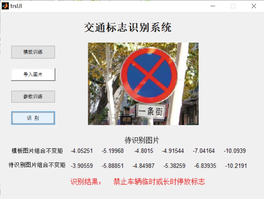
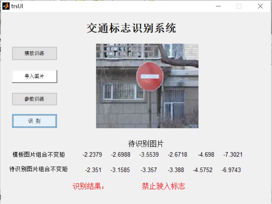
3, Operation results
4, matlab version and references
1 matlab version
2014a
2 references
[1] Cai Limei MATLAB image processing -- theory, algorithm and example analysis [M] Tsinghua University Press, 2020
[2] Yang Dan, Zhao Haibin, long Zhe Detailed explanation of MATLAB image processing example [M] Tsinghua University Press, 2013
[3] Zhou pin MATLAB image processing and graphical user interface design [M] Tsinghua University Press, 2013
[4] Liu Chenglong Proficient in MATLAB image processing [M] Tsinghua University Press, 2015