Definition of fresh agricultural products
Fresh agricultural products refer to primary products such as fresh fruits that can be sold directly on the shelf without further production. At present, fresh agricultural products mainly include fresh vegetables, fruits, flowers, eggs, milk, raw poultry, aquatic products and fresh meat products. These kinds of products occupy a major position in fresh agricultural products. They are traditionally called the three fresh products - fruits and vegetables, meat and aquatic products
research objective
The main research purpose of this paper is to plan the most reasonable vehicle distribution path based on distribution center, traffic route planning and intelligent distribution mode on the basis of reducing logistics distribution cost, improving distribution efficiency and maintaining the freshness and timeliness of fresh agricultural products, so as to achieve the common satisfactory results of both supply and demand. By summarizing and integrating the characteristics of fresh agricultural products and considering the relevant constraints such as distribution time, a more accurate and detailed mathematical model for defining the vehicle routing problem of fresh agricultural products distribution is established, and a more practical and simple solution is found, In order to achieve fresh agricultural products in the distribution process to achieve product preservation and quality, meet customer satisfaction requirements, and achieve the lowest distribution cost and maximize benefits
Research methods and ideas
On the basis of previous research results, this paper understands the relevant knowledge and content of fresh agricultural products distribution, analyzes and further explores its distribution path, and defines the optimization objectives and planning of vehicle path. Specifically, the following research methods are adopted:
(1) Literature method: study the theory of fresh product distribution and vehicle routing with time window by reviewing the relevant literature at home and abroad on two-way logistics distribution, fresh agricultural product transportation, time window solution, vehicle routing planning, etc., so as to provide a strong theoretical basis for the creation of the paper.
(2) Model method: through the analysis and summary of the distribution mode of fresh agricultural products, establish the vehicle route and model suitable for the distribution target of fresh agricultural products, so as to provide a theoretical basis for the development of fresh agricultural products distribution
(3) Simulation analysis method: judge whether it is effective through the data analysis of simulation experiment.
After combining the research methods with the research contents, the research ideas mainly include the following steps:
(1) The distribution mode and related theoretical research status of fresh agricultural products are deeply studied;
(2) Through the analysis of the characteristics and distribution mode of fresh agricultural products, understand its basis and related theories, and further explore its vehicle routing problem on the basis of time window theory.
(3) According to the characteristics of fresh agricultural products and the research of vehicle routing problem, combined with the existing research methods, a vehicle routing model with time window is established, and the genetic algorithm is used to solve the model.
Distribution characteristics of fresh agricultural products
Compared with ordinary product distribution, fresh agricultural products also have different requirements in logistics distribution because of their unique attributes. With the improvement of economic level and consumption level, the distribution market demand of fresh agricultural products is large, and the distribution objects are also different. Generally speaking, the logistics distribution characteristics of fresh agricultural products are as follows:
(1) The distribution cost is high. There are many factors that affect the whole logistics cost in the process of product distribution. For ordinary products, they include labor cost, vehicle consumption and maintenance cost, storage cost, etc. based on their own attributes and characteristics, in addition to the above conventional factors, the distribution cost is also constrained by the following points:
① Loss of the product itself. Fresh agricultural products are perishable and perishable. In the process of distribution, they will inevitably suffer from bumps, muggy, extrusion and other problems, which will inevitably damage the integrity and freshness of the products and cause the loss of the products themselves.
② Storage method. Because fresh agricultural products are easy to be consumed, it will also bring some difficulties to storage in the process of distribution. There are high requirements for technology, mode and storage space. Compared with ordinary products, it is bound to increase the storage cost of products.
(2) Timeliness. Due to the large demand for fresh agricultural products in the market, the types, quantities and characteristics of fresh agricultural products involved in orders for fresh agricultural products in the specific distribution process are different, and there may be multi-objective distribution with different order demanders. At this time, combined with the unique attributes of fresh agricultural products, it is necessary to further improve the distribution speed in the distribution process to ensure the quality of fresh agricultural products The freshness of fresh agricultural products and customers' satisfaction with the distribution of fresh agricultural products
(3) There are many categories. With the improvement of economic level, the types of fresh agricultural products are further enriched with scientific and technological breeding methods, and the market demand for fresh agricultural products tends to be diversified. Especially for orders from small customers, such as families, hotels and small restaurants, the choice of fresh agricultural products is more abundant and diverse in the past, so fresh agricultural products are required In the process of sending the production base to the distribution center and then from the distribution center to the customers, we should enrich the types and distribution methods of fresh commodities, so that customers can have more choices in order to provide better services.
Model constraints
(1) Achieve the customer's satisfaction with the overall distribution service and quality in the required time period;
(2) Achieve customer satisfaction with the quality of fresh agricultural products when delivered;
(3) Limit the loading capacity of each distribution vehicle and do not exceed the loading capacity and capacity of the vehicle;
(4) The initial freshness and loss of each type of fresh agricultural products are consistent;
(5) Achieve customer satisfaction with the type, quality and quantity of fresh agricultural products, and realize the simultaneous distribution of all products;
(6) Each target customer has only one means of transportation to serve them;
(7) The speed change and road congestion during vehicle driving are not considered.
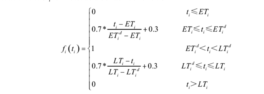
customer satisfaction
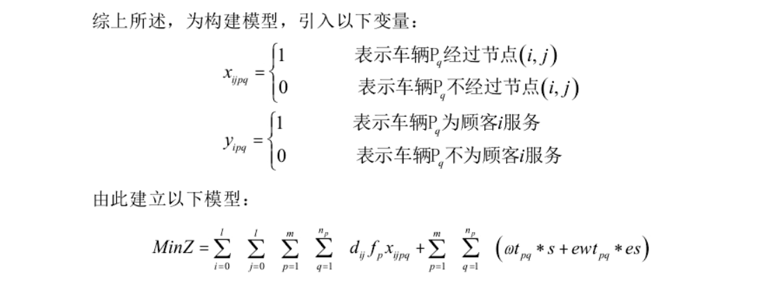
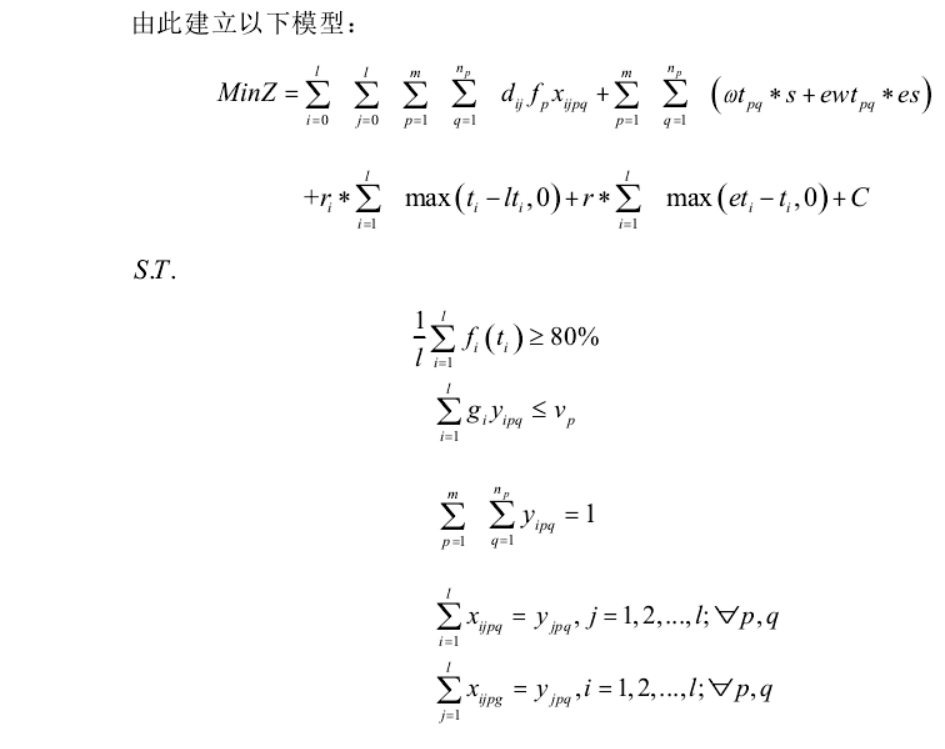
Model
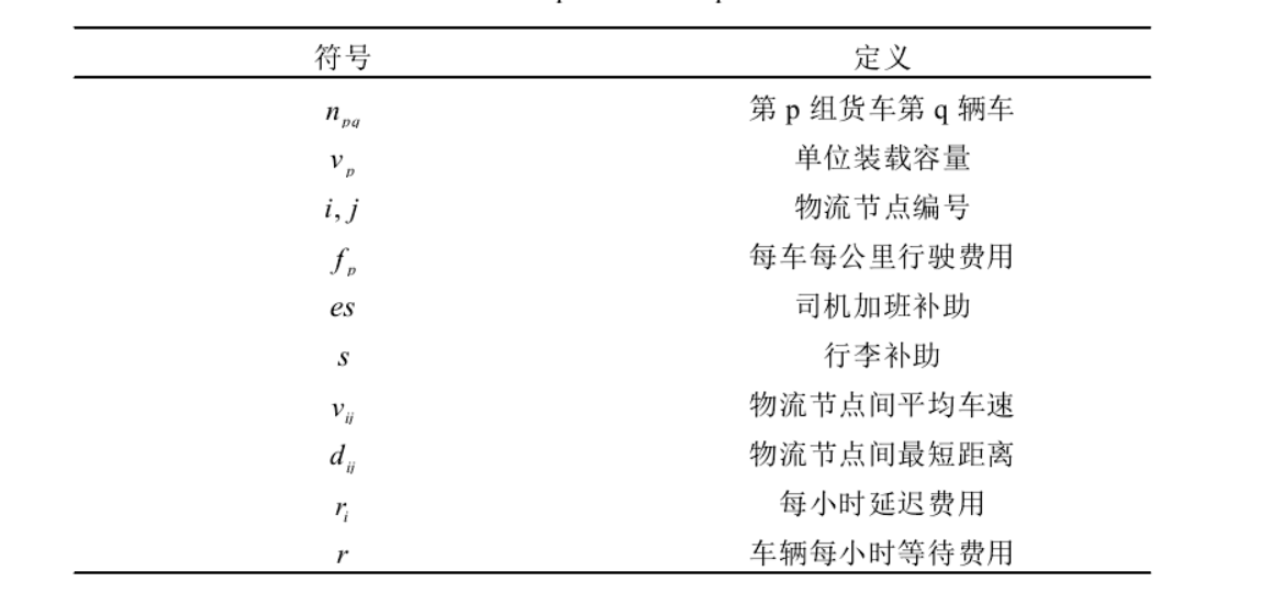
Where:
(5.1) is the objective function, indicating the minimum distribution cost.
(5.2) it is the constraint of customer satisfaction, which means that the average value of customer satisfaction should be above.
(5.3) load capacity constraints for vehicles
(5.4) it is used to ensure that customers only complete the distribution by the q vehicle of group p.
(5.5) and (5.6) represent the only vehicles arriving at a customer, that is, each customer has and only one vehicle to serve him.
main program
clear
clc
close all
tic
%% use importdata This function reads the file
% shuju=importdata('cc101.txt');
load('c101');
shuju=c101;
% bl=importdata('103.txt');
bl=0;
cap=1500;                                                        %Maximum vehicle load
%% Extract data information

E=shuju(1,5);                                                    %Start time of distribution center time window
L=shuju(1,6);                                                    %Distribution center time window end time
zuobiao=shuju(:,2:3);                                       %Coordinates of all points x and y
% vertexs= vertexs./1000;
customer=zuobiao(2:end,:);                                       %Customer coordinates
cusnum=size(customer,1);                                         %Number of customers
v_num=6;                                                        %Maximum number of vehicles used
demands=shuju(2:end,4);                                          %requirement
a=shuju(2:end,5);                                                %Customer time window start time[a[i],b[i]]
b=shuju(2:end,6);                                                %End time of customer time window[a[i],b[i]]
s=shuju(2:end,7);                                                %Service time at customer points
h=pdist(zuobiao);
dist=squareform(h);
dist=dist./1000;%The distance matrix satisfies the triangular relationship and temporarily uses the distance to represent the cost c[i][j]=dist[i][j]
%% Genetic algorithm parameter setting
alpha=100000;                                                       %Penalty function coefficients for violating capacity constraints
belta=900;%Penalty function coefficients for violation of time window constraints
belta2=60;
chesu=30;

NIND=100;                                                       %Population size
MAXGEN=500;                                                     %Number of iterations
Pc=0.9;                                                         %Crossover probability
Pm=0.05;                                                        %Variation probability
GGAP=0.9;                                                       %generation gap(Generation gap)
N=cusnum+v_num-1;                                %Chromosome length=Number of customers+Maximum number of vehicles used-1
% N=cusnum;
%% Initialize population
init_vc=init(cusnum,a,demands,cap);                             %Construct initial solution
Chrom=InitPopCW(NIND,N,cusnum,init_vc);
%% Route and total distance of output random solution
disp('A random value in the initial population:')

[VC,NV,TD,violate_num,violate_cus]=decode(Chrom(1,:),cusnum,cap,demands,a,b,L,s,dist,chesu,bl);
[~,~,bsv]=violateTW(VC,a,b,s,L,dist,chesu,bl);
% disp(['Total distance:',num2str(TD)]);
disp(['Number of vehicles used:',num2str(NV),',Total vehicle distance:',num2str(TD)]);
disp('~~~~~~~~~~~~~~~~~~~~~~~~~~~~~~~~~~~~~~~~~~~~~~~~~~~~~~~~~~~~~~~~')
%% optimization
gen=1;
figure;
hold on;box on
xlim([0,MAXGEN])
title('Optimization process')
xlabel('Algebra')
ylabel('optimal value')
ObjV=calObj(Chrom,cusnum,cap,demands,a,b,L,s,dist,alpha,belta,belta2,chesu,bl);             %Calculate the value of population objective function
preObjV=min(ObjV);
while gen<=MAXGEN
    %% Calculate fitness
    ObjV=calObj(Chrom,cusnum,cap,demands,a,b,L,s,dist,alpha,belta,belta2,chesu,bl);             %Calculate the value of population objective function
    line([gen-1,gen],[preObjV,min(ObjV)]);pause(0.0001)%Drawing optimal function
    preObjV=min(ObjV);
    FitnV=Fitness(ObjV);
    %% choice
    SelCh=Select(Chrom,FitnV,GGAP);
    %% OX Cross operation
    SelCh=Recombin(SelCh,Pc);
    %% variation
    SelCh=Mutate(SelCh,Pm);
    %% New populations of reinsertion Progenies
    Chrom=Reins(Chrom,SelCh,ObjV);
    %% Print current optimal solution
    ObjV=calObj(Chrom,cusnum,cap,demands,a,b,L,s,dist,alpha,belta,belta2,chesu,bl);             %Calculate the value of population objective function
    [minObjV,minInd]=min(ObjV);
    disp(['The first',num2str(gen),'Generation optimal solution:'])
    [bestVC,bestNV,bestTD,best_vionum,best_viocus]=decode(Chrom(minInd(1),:),cusnum,cap,demands,a,b,L,s,dist,chesu,bl);
    disp(['Number of vehicles used:',num2str(bestNV),',Total vehicle distance:',num2str(bestTD)]);
    fprintf('\n')
    %% Update iterations
    gen=gen+1 ;
end
%% Draw the road map of the optimal solution
ObjV=calObj(Chrom,cusnum,cap,demands,a,b,L,s,dist,alpha,belta,belta2,chesu,bl);             %Calculate the value of population objective function
[minObjV,minInd]=min(ObjV);
%% Route and total distance of output optimal solution
disp('Optimal solution:')
bestChrom=Chrom(minInd(1),:);
[bestVC,bestNV,bestTD,best_vionum,best_viocus]=decode(bestChrom,cusnum,cap,demands,a,b,L,s,dist,chesu,bl);
disp(['Number of vehicles used:',num2str(bestNV),',Total vehicle distance:',num2str(bestTD)]);
disp('-------------------------------------------------------------')
[cost,q1,q2,q3,q4,q5,q6]=costFuction(bestVC,a,b,s,L,dist,demands,cap,alpha,belta,belta2,chesu,bl);
%% Draw the final road map
draw_Best(bestVC,zuobiao);
result
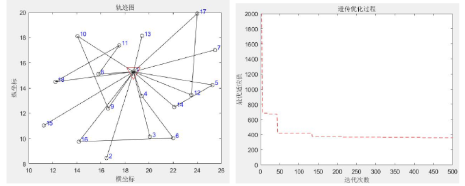
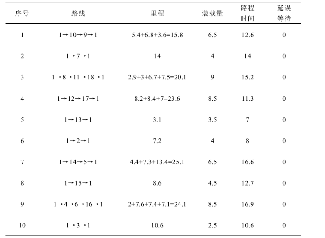
The calculation results show that under the use of 9 vehicles, the optimal feasible solution obtained through operation is {1,8,10,1,2,16,1,3,1,18,15,1,7,1,5,1,4,12,14,1,11,13,17,16,9,1}. After completing the overall distribution task, the corresponding minimum total distribution cost is reduced from 359.3838 yuan of 10 vehicles to 2874416 yuan, and the total mileage is 1297735km. At the same time, the transportation time of each vehicle is relatively average, There is no excessive use of some vehicles, and the transportation time of each vehicle is not long, which is basically about 12 hours, which can maintain the freshness of fresh agricultural products. Through the above comparison, it can be seen that the distribution result of 9 vehicles is better than that of 10 vehicles, and the transportation cost and mileage are better. This means that in the future research process, the use of vehicles can be reasonably arranged while optimizing the distribution vehicle route, so as to further reduce the overall distribution cost and improve the distribution efficiency.
If you need help, V: zhangshu2274