1. Introduction

Principle of Wavelet Transform
Wavelet transform is a time-scale (time-frequency) analysis method for signals. It is a time-frequency localization analysis method where the window size is fixed and the shape can be changed, and the time window and frequency window can be changed. It is characterized by multi-resolution analysis and has the ability to characterize the local characteristics of signals in both time and frequency domains.
Wavelet analysis is known as a "mathematical microscope" because it has higher frequency resolution and lower time resolution in the low frequency part, higher time resolution and lower frequency resolution in the high frequency part. It is this characteristic that makes the wavelet transform adaptive to the signal.
Wavelet analysis, considered the crystallization of half a century's work in harmonic analysis, has been widely used in signal processing, image processing, quantum field theory, seismic exploration, speech recognition and synthesis, music, radar, CT imaging, color copy, fluid turbulence, object recognition, machine vision, mechanical fault diagnosis and monitoring. Sciences such as fractal and digital TV.
In principle, where Fourier analysis is traditionally used, it can be replaced by wavelet analysis. What makes wavelet analysis better than Fourier transform is that it has good localization properties in both time and frequency domains.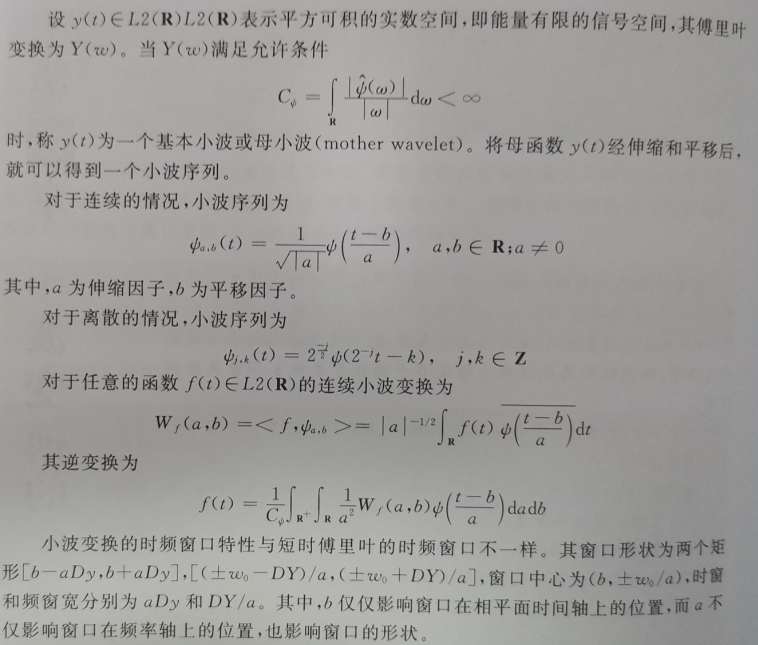

In this way, the time-domain sampling step of the wavelet transform is adjustable for different frequencies: at low frequencies, the time resolution of the wavelet transform is lower and the frequency division rate is higher; At high frequencies, the time resolution of the wavelet transform is higher and the class resolution is lower. This corresponds to the characteristics of slow change of low frequency signal and fast change of high frequency signal.
This is where it is superior to classical and short-time Fourier transforms.

Source Code

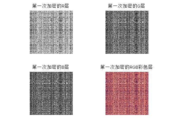
%Confuse rows and columns for the first time encryption of plain text images %%%

clear;

W = imread('lena.tif');

s = size(W);

r = randsample(s(1), s(1));

W1 = W(r, :, :);

c = randsample(s(2), s(2));

W2 = W1(:, c, :);

i = 1; f = 1:length(c);

while i <= length(c)

f(i) = find(c == i);

i = i + 1;

end

P = W2;

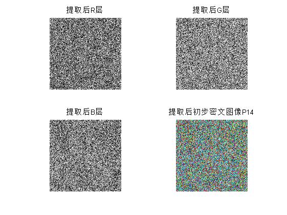
R = P(:,:,1); %Extracting plain text images R Layer Pixels

G = P(:,:,2); %Extracting plain text images G Layer Pixels

B = P(:,:,3); %Extracting plain text images B Layer Pixels

figure(1)

subplot(2,2,1);imshow(R,[]);title('First encrypted R layer');imwrite(R,'R1.tif')

subplot(2,2,2);imshow(G,[]);title('First encrypted G layer');imwrite(G,'G1.tif')

subplot(2,2,3);imshow(B,[]);title('First encrypted B layer');imwrite(B,'B1.tif')

subplot(2,2,4);imshow(P,[]);title('First encrypted RGB Color layer');imwrite(P,'First encrypted RGB Color layer.tif')

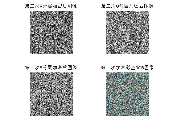
%%%%%%Second Encryption%%%%%

[M,N]=size(R); %utilize Logistic Chaotic Mapping, for R Sequence Encryption for Layered Images

u=3.9;

x0=0.5;

x=x0;

for i=1:100 %100 iterations to achieve full chaos

x=u*x*(1-x);

end

R1=zeros(1,M*N); %Produce one-dimensional chaotic encryption sequence

R1(1)=x;

for i=1:M*N-1

R1(i+1)=u*R1(i)*(1-R1(i));

end

R2=uint8(255*R1); %Normalized Sequence

R3=reshape(R2,M,N); %Convert to two-dimensional chaotic encryption sequence

R4=bitxor(R,R3); %XOR Operation Encryption

imwrite(R4,'R2.tif')


% [M,N]=size(G); %utilize Logistic Chaotic Mapping, for G Sequence Encryption for Layered Images

u=3.9;

x0=0.5;

x=x0;

for i=1:100 %100 iterations to achieve full chaos

x=u*x*(1-x);

end

G1=zeros(1,M*N); %Produce one-dimensional chaotic encryption sequence

G1(1)=x;

for i=1:M*N-1

G1(i+1)=u*G1(i)*(1-G1(i));

end

G2=uint8(255*G1); %Normalized Sequence

G3=reshape(G2,M,N); %Convert to two-dimensional chaotic encryption sequence

G4=bitxor(G,G3); %XOR Operation Encryption

imwrite(G4,'G2.tif')


% [M,N]=size(B); %utilize Logistic Chaotic Mapping, for B Sequence Encryption for Layered Images

u=3.9;

x0=0.5;

x=x0;

for i=1:100 %100 iterations to achieve full chaos

x=u*x*(1-x);

end

B1=zeros(1,M*N); %Produce one-dimensional chaotic encryption sequence

B1(1)=x;

for i=1:M*N-1

B1(i+1)=u*B1(i)*(1-B1(i));

end

B2=uint8(255*B1); %Normalized Sequence

B3=reshape(B2,M,N); %Convert to two-dimensional chaotic encryption sequence

B4=bitxor(B,B3); %XOR Operation Encryption

imwrite(B4,'B2.tif')


%RGB Triple-layer synthesis

P1=cat(3,R4,G4,B4);


figure(2);

subplot(2,2,1);imshow(R4);title('The second time R Layered Encrypted Image');

subplot(2,2,2);imshow(G4);title('The second time G Layered Encrypted Image');

subplot(2,2,3);imshow(B4);title('The second time B Layered Encrypted Image');

subplot(2,2,4);imshow(P1);title('Second encrypted color RGB image');

imwrite(P1,'Second encrypted color RGB image.tif')


%%%%%%%%%%%%%%%%%%%%%%%%%%Embedding ciphertext image into carrier image%%%%%%%%%%%%%%%%%%%

%Read carrier image

F = imread('houlian.tif');

Rf = F(:,:,1); %Extracting carrier image R Layer Pixels

Gf = F(:,:,2); %Extracting carrier image G Layer Pixels

Bf = F(:,:,3); %Carrier for image extraction B Layer Pixels

figure(3);

subplot(2,2,1);imshow(Rf);title('Carrier Image R layer');

subplot(2,2,2);imshow(Gf);title('Carrier Image G layer');

subplot(2,2,3);imshow(Bf);title('Carrier Image B layer');

subplot(2,2,4);imshow(F);title('Carrier Image RGB Color layer');


%take R4,G4,B4 The pixel value is divided into decimal and ten bits

RCV=mod(R4,10);RCD=floor(R4./10);

GCV=mod(G4,10);GCD=floor(G4./10);

BCV=mod(B4,10);BCD=floor(B4./10);


% Layered Wavelet Decomposition of Carrier Image,And embedding

wave_in='db1';

[Rll,Rlh,Rhl,Rhh]=dwt2(Rf,wave_in);

mv=mean(Rll(:));%Find Matrix Rll average value

for i=1:floor(M)

for j=1:floor(N)

if(Rll(i,j)>=mv)

Rlh(i,j)=RCV(i,j);

Rhl(i,j)=RCD(i,j);

else

Rlh(i,j)=RCD(i,j);

Rhl(i,j)=RCV(i,j);

end

end

end


[Gll,Glh,Ghl,Ghh]=dwt2(Gf,wave_in);

mv=mean(Gll(:));%Find Matrix Gll average value

for i=1:floor(M)

for j=1:floor(N)

if(Gll(i,j)>=mv)

Glh(i,j)=GCV(i,j);

Ghl(i,j)=GCD(i,j);

else

Glh(i,j)=GCD(i,j);

Ghl(i,j)=GCV(i,j);

end

end

end


[Bll,Blh,Bhl,Bhh]=dwt2(Bf,wave_in);

mv=mean(Bll(:));%Find Matrix Bll average value

for i=1:floor(M)

for j=1:floor(N)

if(Bll(i,j)>=mv)

Blh(i,j)=BCV(i,j);

Bhl(i,j)=BCD(i,j);

else

Blh(i,j)=BCD(i,j);

Bhl(i,j)=BCV(i,j);

end

end

end


% Inverse Wavelet Transform(idwt)，Get visually safe images FRGB

Fr=idwt2(Rll,Rlh,Rhl,Rhh,wave_in);

Fg=idwt2(Gll,Glh,Ghl,Ghh,wave_in);

Fb=idwt2(Bll,Blh,Bhl,Bhh,wave_in);

Frgb(:,:,1)=Fr;%%Synthesis

Frgb(:,:,2)=Fg;%%Synthesis

Frgb(:,:,3)=Fb;%%Synthesis

Frgb=uint8(Frgb);

figure(4);

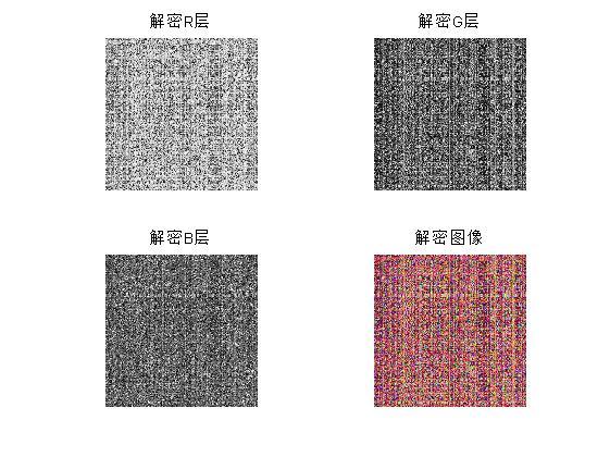
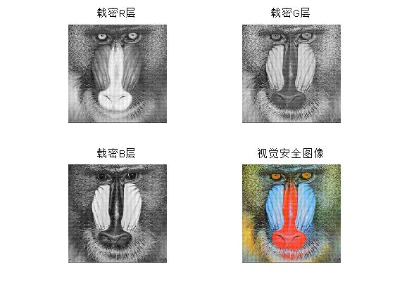
subplot(2,2,1);imshow(Fr,[]);title('Carrier Density R layer');

subplot(2,2,2);imshow(Fg,[]);title('Carrier Density G layer');

subplot(2,2,3);imshow(Fb,[]);title('Carrier Density B layer');

subplot(2,2,4);imshow(uint8(Frgb),[]);title('Visual Safety Images');

imwrite(Frgb,'Visual Safety Images.tif')


%%%%%%%%%%%%%%%%%%%%%%%%%%Extracting plain text ciphertext images from visually secure ciphertext images%%%%%%%%%%%%%%%%%%%

C=Frgb;

%From here, the restore is decomposed first RGB three layers

% close all;

Cr=C(:,:,1);

Cg=C(:,:,2);

Cb=C(:,:,3);

[Rll1,Rlh1,Rhl1,Rhh1]=dwt2(Cr,wave_in);

mv=median(Rll1(:));

RD1=zeros(M,N);RD2=zeros(M,N);%Defines two matrices for decimal and ten bits

for i=1:floor(M)

for j=1:floor(N)

if(Rll1(i,j)>=mv)

RD1(i,j)=Rlh1(i,j);

RD2(i,j)=Rhl1(i,j);

else

RD2(i,j)=Rlh1(i,j);

RD1(i,j)=Rhl1(i,j);

end

end

end

3. Operation results