1, Introduction to particle swarm optimization

1 concept of particle swarm optimization
Particle swarm optimization (PSO) is an evolutionary computing technology, which originates from the research on the predation behavior of birds. The basic idea of particle swarm optimization algorithm is to find the optimal solution through the cooperation and information sharing among individuals in the population
The advantage of PSO is that it is simple and easy to implement, and there is no adjustment of many parameters. At present, it has been widely used in function optimization, neural network training, fuzzy system control and other application fields of genetic algorithm.

2 particle swarm optimization analysis
2.1 basic ideas
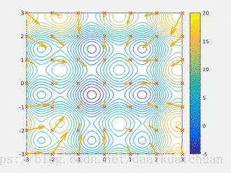
Particle swarm optimization algorithm designs a massless particle to simulate the birds in the bird swarm. The particle has only two attributes: speed and position. Speed represents the speed of movement and position represents the direction of movement. Each particle separately searches for the optimal solution in the search space, records it as the current individual extreme value, shares the individual extreme value with other particles in the whole particle swarm, and finds the optimal individual extreme value as the current global optimal solution of the whole particle swarm, All particles in the particle swarm adjust their speed and position according to the current individual extreme value found by themselves and the current global optimal solution shared by the whole particle swarm. The following dynamic diagram vividly shows the process of PSO algorithm:

2 update rules
PSO is initialized as a group of random particles (random solutions). Then the optimal solution is found by iteration. In each iteration, the particles update themselves by tracking two "extreme values" (pbest, gbest). After finding these two optimal values, the particle updates its speed and position through the following formula.

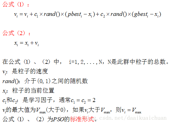
The first part of formula (1) is called [memory item], which indicates the influence of the last speed and direction; the second part of formula (1) is called [self cognition item], which is a vector from the current point to the best point of the particle itself, which indicates that the action of the particle comes from its own experience; the third part of formula (1) is called [group cognition item] is a vector from the current point to the best point of the population, which reflects the cooperation and knowledge sharing among particles. Particles determine the next movement through their own experience and the best experience of their peers. Based on the above two formulas, it forms the standard form of PSO.

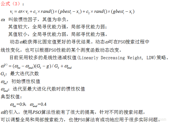
Equations (2) and (3) are considered as standard PSO algorithms.
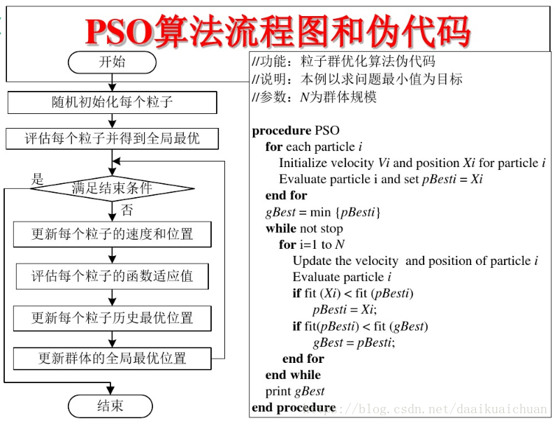
3 PSO algorithm flow and pseudo code

2, Source code

clear
clc
close all
%% Parameter initialization
c1=2.05;
c2=2.05;
maxgen=5000;
sizepop=30;
k=0.6;
% wV=1.1;
wP=1.1;
v=5;
popmax=30;
popmin=-30;

%      pso_option = struct('c1',1.5,'c2',1.7,'maxgen',200,'sizepop',20, ...
%                    'k',0.6,'wV',1,'wP',1,'v',5, ...
%                     'popcmax',100,'popcmin',0.1,'popgmax',10^3,'popgmin',10^(-2));
% c1:The initial value is 1.5,pso Parameter local search capability
% c2:The initial value is 1.7,pso Parameter global search capability
% maxgen:Initially 200,Maximum evolutionary quantity
% sizepop:Initial 20,Maximum population
% k:Initial 0.6(k belongs to [0.1,1.0]),Rate and x Relationship between(V = kX)
% wV:The initial value is 1(wV best belongs to [0.8,1.2]),Elastic coefficient in front of velocity in rate update formula
% wP:The initial value is 1,Elastic coefficient in front of velocity in population renewal formula
% v:Initially 5,SVM Cross Validation parameter
% popcmax:Initially 100,SVM parameter c Maximum value of change in.
% popcmin:Initial 0.1,SVM parameter c Minimum value of change.
% popgmax:Initially 1000,SVM parameter g Maximum value of change in.
% popgmin:Initial 0.01,SVM parameter c Minimum value of change.
D=10;  %%%dimension
Vmax =k*popmax;
Vmin = -Vmax ;

eps =1E-5;

%% Generate initial particles and velocities
pop=zeros(sizepop,D);
V=zeros(sizepop,D);
fitness=zeros(sizepop,1);
for i=1:sizepop
    
    % Randomly generated population and speed
    pop(i,:) = (popmax-popmin)*rand(1,D)+popmin;
    
    V(i,:)=Vmax*rands(1,D);
    
    % Calculate initial fitness
    fitness(i)=myfunc_fit1(pop(i,:));
    
end
Xd_ave0=repmat(sum(pop)/sizepop,sizepop,1);
D_t0=sum((sum((pop-Xd_ave0).^2,2)).^0.5)/sizepop/(popmax-popmin);
wV=1/(1+exp(-12*(D_t0-0.5)));

D_min=D_t0*0.2;

% Find extreme value and extreme point
[global_fitness bestindex]=min(fitness); % Global extremum
local_fitness=fitness;   % Individual extremum initialization

global_x=pop(bestindex,:);   % Global extreme point
local_x=pop;    % Individual extreme point initialization

% Average fitness of each generation population
avgfitness_gen = zeros(maxgen,1);
fit_gen=zeros(maxgen,1);

%% Iterative optimization
for i=1:maxgen
    
    for j=1:sizepop
        
        %Speed update
        V(j,:) = wV*V(j,:) + c1*rand*(local_x(j,:) - pop(j,:)) + c2*rand*(global_x - pop(j,:));
        if find(V(j,:) > Vmax)
            V_maxflag=find(V(j,:) > Vmax);
            V(j,V_maxflag) = Vmax;
        end
        if find(V(j,1) < Vmin)
            V_minflag=find(V(j,1) < Vmin);
            V(j,V_minflag) = Vmin;
        end
        
        %Population regeneration
        pop(j,:)=pop(j,:) + wP*V(j,:);
        if find(pop(j,:) > popmax)
            pop_maxflag=find(pop(j,:) > popmax);
            pop(j,pop_maxflag) = popmax;
        end
        if find(pop(j,:) < popmin)
            pop_minflag=find(pop(j,:) < popmin);
            pop(j,pop_minflag) = popmin;
        end
        
        % Adaptive particle mutation
        if rand>0.5
            k=ceil(2*rand);
            pop(j,k) = (popmax-popmin)*rand + popmin;
        end
        
        %Fitness value
        fitness(j)=myfunc_fit1(pop(j,:));
        
        %Individual optimal update
        if fitness(j) < local_fitness(j)
            local_x(j,:) = pop(j,:);
            local_fitness(j) = fitness(j);
        end
        
%         if fitness(j) == local_fitness(j) && length(pop(j,:) < local_x(j,:))
%             local_flag=find(pop(j,:) < local_x(j,:));
%             local_x(j,local_flag) = pop(j,local_flag);
%             local_fitness(j) = fitness(j);
%         end
        
        %Group optimal update
        if fitness(j) < global_fitness
            global_x = pop(j,:);
            global_fitness = fitness(j);
        end
        function C=PSO_FUNC(X)
global G_AC T_C hour_num Wind_V
C_W=110;   %%%Wind power generation
P_W=100;
u_PW=6;
m_WG=20;
r0=0.06;
v_ci=3; %Cut in wind speed
v_r=12; %Rated wind speed
v_co=25; %Cut off wind speed
P_r=P_W;
V_t=repmat(Wind_V(:,3),52,1);

C_S=0.7;   %%%%Photovoltaic power generation
P_S=0.2;
u_PS=0.009;
m_PV=25;

C_B=0.5;   %%%Battery
u_WB=0.0014;
m_B=5;

sigam_bat=1e-4;   %%%Self discharge rate
N_B=2000;
W_B=0.64;
Wbat_0=0.5*N_B*W_B;
Pbat_max=0.2*N_B*W_B;
Pbat_min=-0.2*N_B*W_B;
Pbat_maxt=Pbat_max;
Pbat_mint=Pbat_min;
Wbat_t=zeros(hour_num,1);
Wbat_t(1)=Wbat_0; %%%Remaining power

Pbat_t=zeros(hour_num,1);
Pbat_t(1)=Pbat_max;


C_d=10;     %%%Diesel generator
u_Pd=0.95;
P=4.62;
Q_d0=0.22;
m_die=10;

P_STC=0.2;
G_STC=1;
K=-0.47;
Tr=298.15;
T_C=T_C+273.15;

P1_t=300;     %%%Peak residential load  KW
Pdes_t=200;   %%%Desalination load   KW
P_des=25;      %%%Rated power of single seawater desalination unit   KW
N_des=8;     %%%Total number of seawater desalination units
G_des=100/24;    %%%The hourly water production of a single unit is 100 t/d
Rwater_t=500/24;  %%%All day water demand on the island   t
Rdes_min=0;
Rdes_max=8*100/24;
eta_c=0.97;

Rdes_t=zeros(hour_num,1);
Rdes_t(1)=Rdes_max;   %%Initial storage 

P_PV=zeros(hour_num,1);
P_WG=zeros(hour_num,1);
P_PVM_t=zeros(hour_num,1);
P_WGM_t=zeros(hour_num,1);
P_net_t=zeros(hour_num,1);
Pdie_t=zeros(hour_num,1);
C_f=0;   %%%Annual cost of diesel
yeushu1=0;
yeushu2=0;
yeushu3=0;
yeushu4=0;
yeushu5=0;
yeushu6=0;
yeushu7=0;
yeushu8=0;
for i=1:hour_num
    P_PV(i)=P_STC*G_AC(i).*(1+K*(T_C(i)-Tr))/G_STC;
    a=P_r/(v_r^3-v_ci^3);
    b=v_ci^3/(v_r^3-v_ci^3);
    if (V_t(i)<v_ci)
        P_WG(i)=0;
    elseif (v_ci<V_t(i)<v_r)
        P_WG(i)=a*V_t(i)^3-b*P_r;
    elseif (v_r<V_t(i)<v_co)
        P_WG(i)=P_r;
    else
        P_WG(i)=0;
    end
    
    if(Rdes_t(i)-Rdes_max>=Rwater_t)
        Ndes_mint=0;
    else
       Ndes_mint=(Rwater_t-(Rdes_t(i)-Rdes_max))/G_des;
    end
    if(Rdes_t(i)+N_des*P_des-Rwater_t<=Rdes_max)
        Ndes_maxt=N_des*P_des;
    else
        Ndes_maxt=(Rdes_max+Rwater_t-Rdes_t(i))/P_des;
    end
    Pdes_mint=Ndes_mint*P_des;
    Pdes_maxt=Ndes_maxt*P_des;
    
    P_PVM_t(i)=P_PV(i);
    P_WGM_t(i)=P_WG(i);
    P_net_t(i)=P_WGM_t(i)+P_PVM_t(i)-P1_t;
    
   if(i>=2)
           Pbat_maxt=min([Pbat_max ((1-sigam_bat)*Wbat_t(i)-((1-sigam_bat)*Wbat_t(i)+Pbat_t(i)))*eta_c]);
           Pbat_mint=max([Pbat_min ((1-sigam_bat)*Wbat_t(i)-((1-sigam_bat)*Wbat_t(i)+Pbat_t(i)))/eta_c]);
   end   

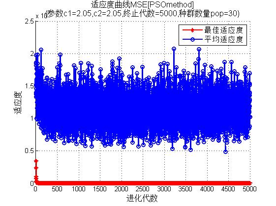
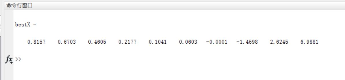
3, Operation results

4, matlab version and references

1 matlab version
2014a

2 references
[1] Steamed stuffed bun Yang, Yu Jizhou, Yang Shan Intelligent optimization algorithm and its MATLAB example (2nd Edition) [M]. Electronic Industry Press, 2016
[2] Zhang Yan, Wu Shuigen MATLAB optimization algorithm source code [M] Tsinghua University Press, 2017