I. Introduction

This paper includes three parts: 1) introduction, 2) introduction and code implementation of image change technology, 3) digital watermarking technology and code implementation based on image transformation technology.

Digital watermarking is an effective technology for copyright protection and data security maintenance of digital products. It is not only an important branch in the field of information hiding, but also a useful supplementary technology of cryptography. In recent years, it has attracted extensive attention. Image invisible watermarking is one of the most important research directions. According to the embedding position, it can be divided into spatial domain methods and transform domain methods (DCT, DFT, DWT, etc.). In order to make the watermark information more robust (the ability to resist attacks), many scholars use the embedding method in the transform domain. In the previous two blogs, I related to the digital watermarking methods and algorithms of DCT. Next, I will introduce the digital watermarking methods and code implementation based on three basic image transformation technologies: DCT, DFT and DWT.

2, DFT, DCT, DWT image transformation technology

Image transformation technology is the transformation of the original image in order to make the image represented by orthogonal function or orthogonal matrix. The transformation is two-dimensional linear reversible. The original image is generally called spatial domain image, The transformed image is called the transformed domain image (also known as frequency domain), the image in the conversion domain can be inversely transformed into a spatial domain image. After image transformation, on the one hand, it can more effectively reflect the characteristics of the image itself, on the other hand, it can also concentrate energy on a small amount of data, which is more conducive to image storage, transmission and processing. From a mathematical point of view, image transformation is to express the pixels in the image as "another form" To meet the actual needs, the transformed graph is needed in most cases The image is inversely transformed to obtain the processed image. This transformation can also be applied to other problems related to physics or mathematics, and other forms of variables can be used. In the field of digital watermarking, the commonly used basic image transformation technologies include Fourier transform (DFT), discrete cosine transform (DCT) and wavelet transform (DWT).

2.1 image Fourier transform (DFT)

Fourier transform is a transformation relationship between "signal" with time as independent variable and "frequency spectrum" function with frequency domain as independent variable. In a purely mathematical sense, Fourier transform transforms an image function into a series of periodic functions; From the physical effect, Fourier transform transforms the image from spatial domain to frequency domain, and its inverse transform transforms the image from frequency domain to spatial domain. In fact, the two-dimensional Fourier transform of the image is used to obtain the spectrum diagram, which is the distribution diagram of the image gradient. The bright spots with different light and shade seen on the Fourier spectrum diagram are actually the strength of the difference between a -- point on the image and its neighborhood point, that is, the size of the gradient, that is, the frequency of the point. If there are more dark points in the spectrum, the actual image is relatively soft; on the contrary, if there are more bright points in the spectrum, the actual image must be sharp, with clear boundaries and large differences in pixels on both sides of the boundary.

Fourier transform includes one-dimensional continuous Fourier transform, two-dimensional continuous Fourier transform, one-dimensional discrete Fourier transform and two-dimensional discrete Fourier transform. Two dimensional discrete Fourier transform is commonly used in the field of image processing. The definition is as follows (1):

                                                                                                       (1)

Where u = 0, 1, M-1;   v = 0, 1, ... , N-1 . The two-dimensional inverse discrete Fourier transform of F (u, v) is defined as the following equation (2):
                                                                                                 (2)                  

The two-dimensional Fourier result of the image is usually in complex form, so the result is squared in the process of image processing. For the specific mathematical calculation formula and the definition of other three Fourier changes, please refer to digital image processing - Gonzalez.

The definition is an abstract expression of the Fourier transform process, but what is the implementation of the image? Next, we use MATLAB tools to carry out the Fourier transform of the image. The codes and results are as follows:

1. close all;

2. clear all;

3. clc;

4. I = imread('pepper.bmp');

5. J = rgb2gray(I);

6. K_1 = fft2(J);

7. L_1 = abs(K_1/256);

8. K_2 = fftshift(K_1);

9. L_2 = abs(K_2/256);

10. figure;

11. subplot(2,2,1);

12. imshow(I); title('original image ');

13. subplot(2,2,2);

14. imshow(J); title('grayscale image ');

15. subplot(2,2,3);

16. imshow(uint8(L_1)); title('fourier spectrum of gray image ');

17. subplot(2,2,4);

18. imshow(uint8(L_2)); title('spectrum after translation ');

The operation results are shown in the figure below:

Fig. 1 example of image Fourier transform

       

2.2 discrete cosine transform (DCT)

Discrete cosine transform (DCT) is a set of cosine functions with different frequencies and amplitudes to approximate an image. In fact, it is the real part of Fourier transform. For an image, most of the visual information of discrete cosine variable is concentrated on a few transform coefficients. Therefore, discrete cosine variable is a common transform coding method for data compression. It can concentrate the energy of high correlation data, which makes it very suitable for image compression. For example, discrete cosine transform is used in JPEG format of international compression standard.

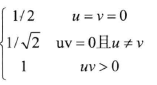
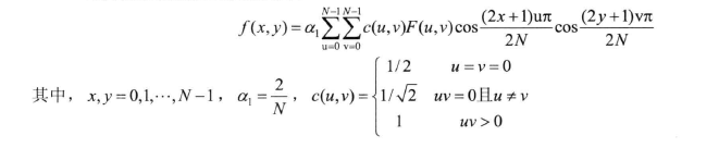
In the process of Fourier transform, if the expanded function is a real even function, then its Fourier transform only contains cosine term. Based on the characteristics of Fourier transform, discrete cosine transform is proposed. DCT transform first transforms the image function into an even function form, and then carries out two-dimensional discrete Fourier transform. Therefore, DCT transform can be regarded as a simplified Fourier transform. The discrete cosine transform leaf is divided into one-dimensional discrete cosine transform and two-dimensional discrete cosine transform. Two dimensional change is used in image processing, so its two-dimensional definition is introduced. For other definitions, please refer to digital image processing - Gonzalez. The two-dimensional discrete cosine transform is defined as follows:

                                                                  (3)

Among them,   

Definition of two-dimensional inverse discrete cosine transform:

                                               (4)

Fourier transform of image with MATLAB tool. The codes and results are as follows:

1. close all;

2. clear all;

3. clc;

4. I = imread ('boats.bmp');

5. J = dct2(I);

6. figure('Name ',' discrete cosine transform ');

7. subplot(1,2,1);

8. imshow(I); title('original image ');

9. subplot(1,2,2);

10. imshow(log(abs(J))); title('discrete cosine transform coefficient image ');

The operation results are shown in Figure 2 below:

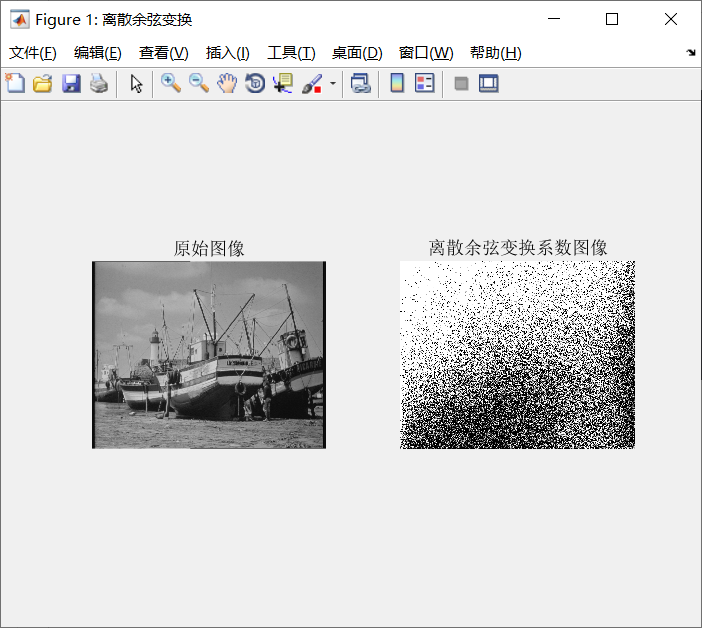
Fig. 2 example of discrete cosine transform

   

2.3 wavelet transform (DWT)

Wavelet transform is a breakthrough in Fourier transform and short-time Fourier transform. Its change is that the infinite trigonometric function basis is replaced by a finite length attenuated wavelet. There are many theories of wavelet transform. For more information, please refer to the relevant chapters of digital image processing - Gonzalez. The following explains wavelet transform from a simple perspective.

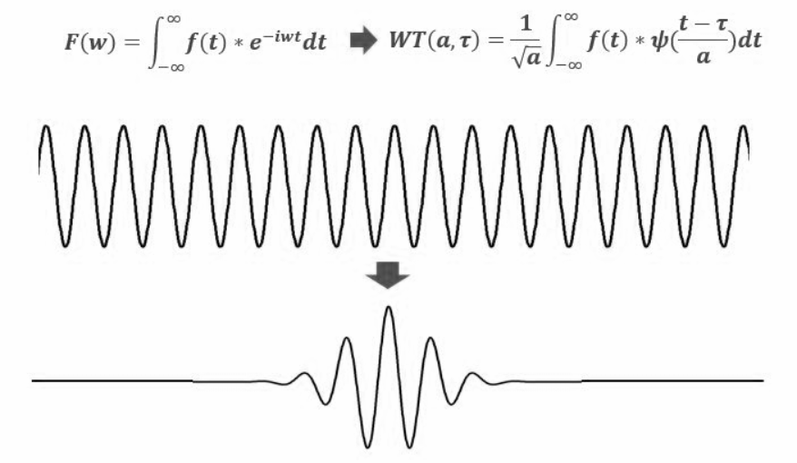
It can also be seen from the above figure why it is called wavelet, and its waveform is small.

The definition formula of one-dimensional continuous wavelet is:

                                                                                                           (5)

Continuous wavelet transform has the following important properties: linearity, translation invariance and redundancy

Several mother wavelet family functions are provided in the MATLAB wavelet transform toolbox, as shown in the table below. Different mother wavelets have different characteristics and different image processing results.

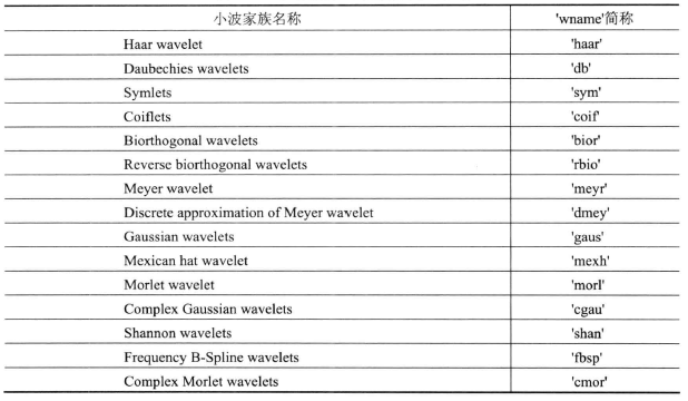
Table 1 mother wavelet of wavelet transform

function varargout = manit1(varargin)
% MANIT1 M-file for manit1.fig
%      MANIT1, by itself, creates a new MANIT1 or raises the existing
%      singleton*.
%
%      H = MANIT1 returns the handle to a new MANIT1 or the handle to
%      the existing singleton*.
%
%      MANIT1('CALLBACK',hObject,eventData,handles,...) calls the local
%      function named CALLBACK in MANIT1.M with the given input arguments.
%
%      MANIT1('Property','Value',...) creates a new MANIT1 or raises the
%      existing singleton*.  Starting from the left, property value pairs are
%      applied to the GUI before manit1_OpeningFcn gets called.  An
%      unrecognized property name or invalid value makes property application
%      stop.  All inputs are passed to manit1_OpeningFcn via varargin.
%
%      *See GUI Options on GUIDE's Tools menu.  Choose "GUI allows only one
%      instance to run (singleton)".
%
% See also: GUIDE, GUIDATA, GUIHANDLES

% Edit the above text to modify the response to help manit1

% Last Modified by GUIDE v2.5 14-Jun-2015 10:32:30

% Begin initialization code - DO NOT EDIT
gui_Singleton = 1;
gui_State = struct('gui_Name',       mfilename, ...
                   'gui_Singleton',  gui_Singleton, ...
                   'gui_OpeningFcn', @manit1_OpeningFcn, ...
                   'gui_OutputFcn',  @manit1_OutputFcn, ...
                   'gui_LayoutFcn',  [] , ...
                   'gui_Callback',   []);
if nargin && ischar(varargin{1})
    gui_State.gui_Callback = str2func(varargin{1});
end

if nargout
    [varargout{1:nargout}] = gui_mainfcn(gui_State, varargin{:});
else
    gui_mainfcn(gui_State, varargin{:});
end
% End initialization code - DO NOT EDIT


% --- Executes just before manit1 is made visible.
function manit1_OpeningFcn(hObject, eventdata, handles, varargin)
% This function has no output args, see OutputFcn.
% hObject    handle to figure
% eventdata  reserved - to be defined in a future version of MATLAB
% handles    structure with handles and user data (see GUIDATA)
% varargin   command line arguments to manit1 (see VARARGIN)

% Choose default command line output for manit1
handles.output = hObject;

% Update handles structure
guidata(hObject, handles);

% UIWAIT makes manit1 wait for user response (see UIRESUME)
% uiwait(handles.figure1);


% --- Outputs from this function are returned to the command line.
function varargout = manit1_OutputFcn(hObject, eventdata, handles) 
% varargout  cell array for returning output args (see VARARGOUT);
% hObject    handle to figure
% eventdata  reserved - to be defined in a future version of MATLAB
% handles    structure with handles and user data (see GUIDATA)

% Get default command line output from handles structure
varargout{1} = handles.output;


% --- Executes on button press in browsecoverimg.
function browsecoverimg_Callback(hObject, eventdata, handles)
% hObject    handle to browsecoverimg (see GCBO)
% eventdata  reserved - to be defined in a future version of MATLAB
% handles    structure with handles and user data (see GUIDATA)
[filename, pathname] = uigetfile({'*.jpg';'*.bmp';'*.gif';'*.*'}, 'Pick an Image File');
S = imread([pathname,filename]);
S=imresize(S,[512,512]);
axes(handles.axes1)
imshow(S)
title('Cover Image')
set(handles.text3,'string',filename)
handles.S=S;
guidata(hObject,handles)

% --- Executes on button press in browsemsg.
function browsemsg_Callback(hObject, eventdata, handles)
% hObject    handle to browsemsg (see GCBO)
% eventdata  reserved - to be defined in a future version of MATLAB
% handles    structure with handles and user data (see GUIDATA)
[filename, pathname] = uigetfile({'*.bmp';'*.jpg';'*.gif';'*.*'}, 'Pick an Image File');
msg = imread([pathname,filename]);
axes(handles.axes2)
imshow(msg)
title('Input Message')
set(handles.text4,'string',filename)
handles.msg=msg;
guidata(hObject,handles)

% --- Executes on button press in DWT.
function DWT_Callback(hObject, eventdata, handles)
% hObject    handle to DWT (see GCBO)
% eventdata  reserved - to be defined in a future version of MATLAB
% handles    structure with handles and user data (see GUIDATA)
message=handles.msg;
cover_object=handles.S;
k=10;
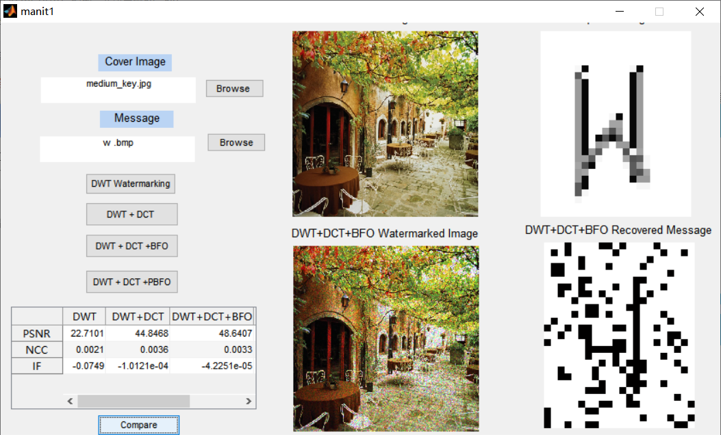
[watermrkd_img,PSNR,IF,NCC,recmessage]=dwt(cover_object,message,k);
axes(handles.axes3)
imshow(watermrkd_img)
title('Watermarked Image')
axes(handles.axes4)
imshow(recmessage)
title('Recovered Message')
a=[PSNR,NCC,IF]';
t=handles.uitable1;
set(t,'Data',a)
handles.a=a;
guidata(hObject,handles)

% --- Executes on button press in DWTDCT.
function DWTDCT_Callback(hObject, eventdata, handles)
% hObject    handle to DWTDCT (see GCBO)
% eventdata  reserved - to be defined in a future version of MATLAB
% handles    structure with handles and user data (see GUIDATA)
a=handles.a;
message=handles.msg;
cover_object=handles.S;
k=10;
[watermrkd_img,recmessage,PSNR,IF,NCC1] = dwtdct(cover_object,message,k);
axes(handles.axes3)
imshow(watermrkd_img)
title('DWT+DCT Watermarked Image')
axes(handles.axes4)
imshow(recmessage)
title('DWT+DCT Recovered Message')
b=[PSNR,NCC1,IF]';
t=handles.uitable1;
set(t,'Data',[a b])
handles.b=b;
guidata(hObject,handles)

% --- Executes on button press in DWTDCTBFO.
function DWTDCTBFO_Callback(hObject, eventdata, handles)
% hObject    handle to DWTDCTBFO (see GCBO)
% eventdata  reserved - to be defined in a future version of MATLAB
% handles    structure with handles and user data (see GUIDATA)
a=handles.a;
b=handles.b;
message=handles.msg;
cover_object=handles.S;
[watermrkd_img,recmessage,PSNR,IF,NCC,pbest] = BG(cover_object,message);
axes(handles.axes3)
imshow(watermrkd_img)
title('DWT+DCT+BFO Watermarked Image')
axes(handles.axes4)
imshow(recmessage)
title('DWT+DCT+BFO Recovered Message')
c=[PSNR,NCC,IF]';
t=handles.uitable1;
set(t,'Data',[a b c])
handles.c=c;
guidata(hObject,handles)

% --- Executes on button press in pushbutton6.
function pushbutton6_Callback(hObject, eventdata, handles)
% hObject    handle to pushbutton6 (see GCBO)
% eventdata  reserved - to be defined in a future version of MATLAB
% handles    structure with handles and user data (see GUIDATA)
a=handles.a;
b=handles.b;
c=handles.c;
d=handles.d;
PSNR=[a(1),b(1),c(1),d(1) ];
NCC=[a(2),b(2),c(2),d(2)];
IF=[a(3),b(3),c(3),d(3)];
figure
bar(PSNR)
set(gca,'XTickLabel',' ');
ylabel('PSNR')
text(1,0,'DWT','Rotation',260,'Fontsize',8);
text(2,0,'DWT+DCT','Rotation',260,'Fontsize',8);
text(3,0,'DWT+DCT+BFO','Rotation',260,'Fontsize',8);
text(4,0,'DWT+DCT+PBFO','Rotation',260,'Fontsize',8);
[t]=get(gca,'position');
set(gca,'position',[t(1) 0.31 t(3) 0.65])
title('Bar Graph Comparison of PSNR')
%%%%
figure
bar(NCC)
set(gca,'XTickLabel',' ');
ylabel('NCC')
text(1,0,'DWT','Rotation',260,'Fontsize',8);
text(2,0,'DWT+DCT','Rotation',260,'Fontsize',8);
text(3,0,'DWT+DCT+BFO','Rotation',260,'Fontsize',8);
text(4,0,'DWT+DCT+PBFO','Rotation',260,'Fontsize',8);
[t]=get(gca,'position');
set(gca,'position',[t(1) 0.31 t(3) 0.65])
title('Bar Graph Comparison of NCC')

% --- Executes on button press in DWTDCTPBFO.
function DWTDCTPBFO_Callback(hObject, eventdata, handles)
% hObject    handle to DWTDCTPBFO (see GCBO)
% eventdata  reserved - to be defined in a future version of MATLAB
% handles    structure with handles and user data (see GUIDATA)
a=handles.a;
b=handles.b;
c=handles.c;
message=handles.msg;
cover_object=handles.S;
[watermrkd_img,recmessage,PSNR,IF,NCC,pbest] =BG_PSO(cover_object,message);
axes(handles.axes3)
imshow(watermrkd_img)
title('DWT+DCT+PBFO Watermarked Image')
axes(handles.axes4)
imshow(recmessage)
title('DWT+DCT+PBFO Recovered Message')
d=[PSNR,NCC,IF]';
t=handles.uitable1;
set(t,'Data',[a b c d])
handles.d=d;
guidata(hObject,handles)

​