1, Introduction to cuckoo algorithm

Cuckoo algorithm is called Cuckoo search (CS algorithm) in English. First of all, let's introduce the English meaning of this algorithm. Cuckoo means cuckoo bird. What is cuckoo bird? It is a bird called cuckoo, o(∩∩) o. this bird's mother is very lazy. She lays her own eggs and doesn't raise them herself. Generally, she throws her baby into the nest of other kinds of birds. However, after hatching, when I met the smart bird mother, I knew it was not my own, and I was directly killed by the bird mother. So in order to protect their lives, these cuckoo babies imitate the songs of other kinds of birds, so that the mother bird with very low IQ or EQ mistakenly thinks it is her own baby, so it will survive.
Cuckoo search (CS) is an optimization algorithm proposed by Xin She Yang and Suash Deb in Cuckoo Search via Levy Flights in 2009. Cuckoo search is a combination of cuckoo nest parasitism and Levy flight (Levy Flights) mode swarm intelligence search technology, through random walk search to get an optimal nest to hatch their own eggs. This method can achieve an efficient optimization mode.

Nest parasitism of cuckoo

2 Levi flight

Figure 1 Schematic diagram of simulated Levi flight trajectory

3 implementation process of cuckoo search algorithm

2, Partial source code

function s=simplebounds(s,Lb,Ub)
  % Apply the lower bound
  ns_tmp=s;
  I=ns_tmp<Lb;
  ns_tmp(I)=Lb(I);
  
  % Apply the upper bounds 
  J=ns_tmp>Ub;
  ns_tmp(J)=Ub(J);
  % Update this new move 
  s=ns_tmp;
end
function errorn = fun(x)
%This function is used to calculate the fitness value
load data X
[n,m]=size(X);
for i=1:n
    y(i,1)=sum(X(1:i,1));
    y(i,2)=sum(X(1:i,2));
    y(i,3)=sum(X(1:i,3));
    y(i,4)=sum(X(1:i,4));
    y(i,5)=sum(X(1:i,5));
    y(i,6)=sum(X(1:i,6));
end

%% Network parameter initialization
a=0.2+x(1)/2;
b1=0.2+x(2)/2;
b2=0.2+x(3)/2;
b3=0.2+x(4)/2;
b4=0.2+x(5)/2;
b5=0.2+x(6)/2;

%% Learning rate initialization
u1=0.0015;
u2=0.0015;
u3=0.0015;
u4=0.0015;
u5=0.0015;

%% Weight threshold initialization
t=1;
w11=a;
w21=-y(1,1);
w22=2*b1/a;
w23=2*b2/a;
w24=2*b3/a;
w25=2*b4/a;
w26=2*b5/a;
w31=1+exp(-a*t);
w32=1+exp(-a*t);
w33=1+exp(-a*t);
w34=1+exp(-a*t);
w35=1+exp(-a*t);
w36=1+exp(-a*t);
theta=(1+exp(-a*t))*(b1*y(1,2)/a+b2*y(1,3)/a+b3*y(1,4)/a+b4*y(1,5)/a+b5*y(1,6)/a-y(1,1));

kk=1;

%% Cyclic iteration
for j=1:10
%Cyclic iteration
E(j)=0;
for i=1:30
    
    %% Network output calculation
    t=i;
    LB_b=1/(1+exp(-w11*t));   %LB Layer output
    LC_c1=LB_b*w21;           %LC Layer output
    LC_c2=y(i,2)*LB_b*w22;    %LC Layer output
    LC_c3=y(i,3)*LB_b*w23;    %LC Layer output
    LC_c4=y(i,4)*LB_b*w24;    %LC Layer output
    LC_c5=y(i,5)*LB_b*w25;    %LC Layer output
    LC_c6=y(i,6)*LB_b*w26;    %LC Layer output 
    LD_d=w31*LC_c1+w32*LC_c2+w33*LC_c3+w34*LC_c4+w35*LC_c5+w36*LC_c6;    %LD Layer output
    theta=(1+exp(-w11*t))*(w22*y(i,2)/2+w23*y(i,3)/2+w24*y(i,4)/2+w25*y(i,5)/2+w26*y(i,6)/2-y(1,1));   %threshold 
    ym=LD_d-theta;   %Network output value
    yc(i)=ym;  %Fitting value
    
    %% Weight correction
    error=ym-y(i,1);      %calculation error
    E(j)=E(j)+abs(error);    %Error summation       
    error1=error*(1+exp(-w11*t));     %calculation error
    error2=error*(1+exp(-w11*t));     %calculation error
    error3=error*(1+exp(-w11*t));
    error4=error*(1+exp(-w11*t));
    error5=error*(1+exp(-w11*t));
    error6=error*(1+exp(-w11*t));
    error7=(1/(1+exp(-w11*t)))*(1-1/(1+exp(-w11*t)))*(w21*error1+w22*error2+w23*error3+w24*error4+w25*error5+w26*error6);
    
    %Modify weight
    w22=w22-u1*error2*LB_b;
    w23=w23-u2*error3*LB_b;
    w24=w24-u3*error4*LB_b;
    w25=w25-u4*error5*LB_b;
    w26=w26-u5*error6*LB_b;
    w11=w11+a*t*error7;
end
end  
%Predict according to the trained grey neural network
for i=1:10
    t=i;
    LB_b=1/(1+exp(-w11*t));   %LB Layer output
    LC_c1=LB_b*w21;           %LC Layer output
    LC_c2=y(i,2)*LB_b*w22;    %LC Layer output
    LC_c3=y(i,3)*LB_b*w23;    %LC Layer output
    LC_c4=y(i,4)*LB_b*w24;    %LC Layer output
    LC_c5=y(i,5)*LB_b*w25;
    LC_c6=y(i,6)*LB_b*w26;
    LD_d=w31*LC_c1+w32*LC_c2+w33*LC_c3+w34*LC_c4+w35*LC_c5+w36*LC_c6;    %LD Layer output
    theta=(1+exp(-w11*t))*(w22*y(i,2)/2+w23*y(i,3)/2+w24*y(i,4)/2+w25*y(i,5)/2+w26*y(i,6)/2-y(1,1));   %threshold 
    ym=LD_d-theta;   %Network output value
    yc(i)=ym;
end
yc=yc*10000;
y(:,1)=y(:,1)*10000;

%Calculate forecast monthly demand
for j=30:-1:2
    ys(j)=(yc(j)-yc(j-1));
end
errorn=sum(abs(ys(2:30)-X(2:30,1)'*10000));
end
function nest=get_cuckoos(nest,best,Lb,Ub)
% Levy flights
n=size(nest,1);
beta=3/2;
sigma=(gamma(1+beta)*sin(pi*beta/2)/(gamma((1+beta)/2)*beta*2^((beta-1)/2)))^(1/beta);

for j=1:n,
    s=nest(j,:);
    % This is a simple way of implementing Levy flights
    % For standard random walks, use step=1;
    %% Levy flights by Mantegna's algorithm
    u=randn(size(s))*sigma;
    v=randn(size(s));
    step=u./abs(v).^(1/beta);
  
    % In the next equation, the difference factor (s-best) means that 
    % when the solution is the best solution, it remains unchanged.     
    stepsize=0.01*step.*(s-best);
    % Here the factor 0.01 comes from the fact that L/100 should the typical
    % step size of walks/flights where L is the typical lenghtscale; 
    % otherwise, Levy flights may become too aggresive/efficient, 
    % which makes new solutions (even) jump out side of the design domain 
    % (and thus wasting evaluations).
    % Now the actual random walks or flights
    s=s+stepsize.*randn(size(s));
   % Apply simple bounds/limits
   nest(j,:)=simplebounds(s,Lb,Ub);
   fitness(j)=fun(nest(j,:));
end

% Find the current best
[fmin,K]=min(fitness) ;
best=nest(K,:);

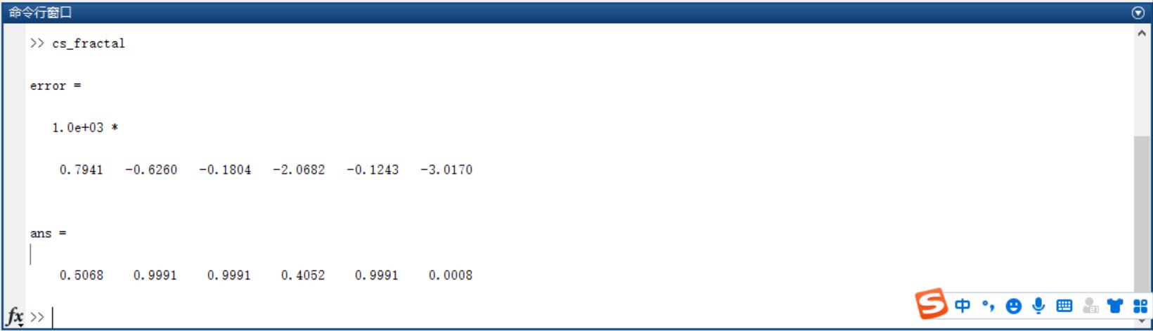
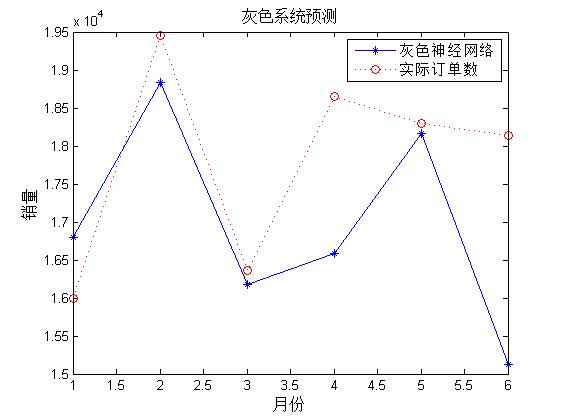
3, Operation results

4, matlab version and references

1 matlab version
2014a

2 references
[1] Steamed stuffed bun Yang, Yu Jizhou, Yang Shan Intelligent optimization algorithm and its MATLAB example (2nd Edition) [M]. Electronic Industry Press, 2016
[2] Zhang Yan, Wu Shuigen MATLAB optimization algorithm source code [M] Tsinghua University Press, 2017
[3] Zhou pin MATLAB neural network design and application [M] Tsinghua University Press, 2013
[4] Chen Ming MATLAB neural network principle and example refinement [M] Tsinghua University Press, 2013
[5] Fang Qingcheng MATLAB R2016a neural network design and application 28 case studies [M] Tsinghua University Press, 2018