Visual introduction of RBF

Many articles on the network must speak better about the specific principle of RBF than I do, so I don't need to talk. Here is only some intuitive understanding of RBF network

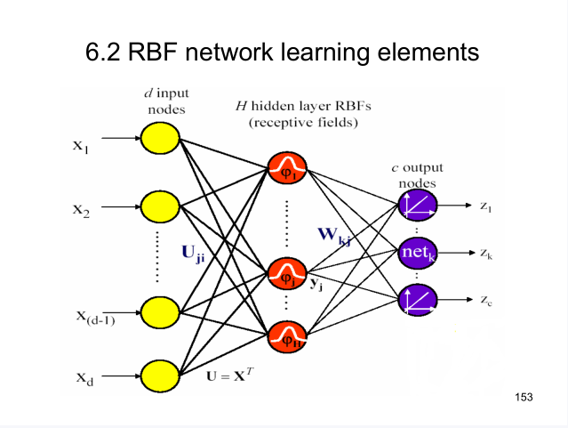
1 RBF is a two-layer network

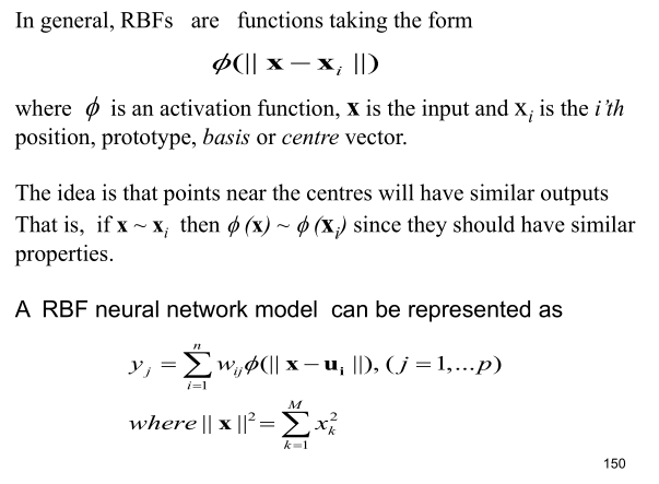
Yes, RBF is not complex in structure. There are only two layers: hidden layer and output layer. The model can be mathematically expressed as:
y j = ∑ i = 1 n w i j ϕ ( ∥ x − u i ∥ 2 ) , ( j = 1 , ... , p ) y_j = \sum_{i=1}^n w_{ij} \phi(\Vert x - u_i\Vert^2), (j = 1,\dots,p)yj​=i=1∑n​wij​ϕ(∥x−ui​∥2),(j=1,...,p)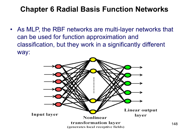

The hidden layer of RBF is a nonlinear mapping

The common activation function of RBF hidden layer is Gaussian function:
ϕ ( ∥ x − u ∥ ) = e − ∥ x − u ∥ 2 σ 2 \phi(\Vert x - u\Vert) = e^{-\frac{\Vert x-u\Vert^2}{\sigma^2}}ϕ(∥x−u∥)=e−σ2∥x−u∥2​

3 RBF output layer is linear

The basic idea of RBF is to transform the data into high-dimensional space and make it linearly separable in high-dimensional space

The RBF hidden layer transforms the data into a high-dimensional space (generally high-dimensional). It is considered that there is a high-dimensional space in which the data can be linearly separable. Therefore, the output layer is linear. This is the same as the idea of the kernel method. Here is an example from the teacher's PPT: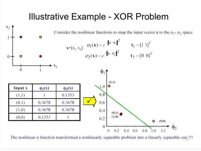

In the above example, the original data is transformed into another two-dimensional space with Gaussian function. In this space, the XOR problem is solved. It can be seen that the converted space is not necessarily higher dimensional than the original.

RBF learning algorithm

For the RBF network in the figure above, the unknowns are: center vector u i u_iui, constant in Gaussian function σ \ sigma σ， Output layer weight W WW.
The whole process of learning algorithm is roughly shown in the figure below: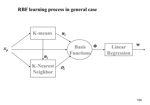

It can be described as:

1. Using kmeans algorithm to find the center vector u i u_iui​
2. Using kNN(K nearest neighbor)rule to calculate σ \ sigma σ
   σ i = 1 K ∑ k = 1 K ∥ u k − u i ∥ 2 \sigma_i = \sqrt{\frac{1}{K}\sum_{k=1}^K \Vert u_k - u_i\Vert^2}σi​=K1​k=1∑K​∥uk​−ui​∥2​
3. WW can be obtained by least square method

Lazy RBF

You can see that the original RBF is very troublesome, both kmeans and knn. Later, someone proposed lazy RBF, which doesn't need kmeans to find the center vector, and takes each data of the training set as the center vector. In this case, the kernel matrix Φ \ Phi Φ Is a square matrix, and as long as the data in training are different, the kernel matrix Φ \ Phi Φ It's reversible. This method is indeed lazy. The disadvantage is that if the training set is large, it will lead to kernel matrix Φ \ Phi Φ The number of training sets should be greater than the dimension of each training data.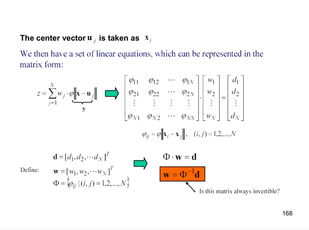

Realization of RBF neural network with MATLAB

The RBF implemented below has only one output for your reference. For multiple outputs, it is also very simple, that is, the WWW has become multiple, which is not implemented here.

demo.m trained and predicted RBF for XOR data, showing the whole process. The last few lines of code are used for training and prediction in the form of encapsulation.

 
% Chaotic time series rbf forecast(One step prediction) -- Main function
clc
clear all
close all
 
%--------------------------------------------------------------------------
% Generating chaotic sequence
% dx/dt = sigma*(y-x)
% dy/dt = r*x - y - x*z
% dz/dt = -b*z + x*y
 
sigma = 16;             % Lorenz Equation parameters a
b = 4;                  %                 b
r = 45.92;              %                 c            
 
y = [-1,0,1];           % starting point (1 x 3 Row vector of)
h = 0.01;               % integration time step 
 
k1 = 30000;             % Number of previous iterations
k2 = 5000;              % Number of subsequent iterations
 
Z = LorenzData(y,h,k1+k2,sigma,r,b);
X = Z(k1+1:end,1);      % time series
X = normalize_a(X,1);   % The signal is normalized to a mean of 0,The amplitude is 1
 
%--------------------------------------------------------------------------
% Related parameters
 
t = 1;                  % time delay
d = 3;                  % embedding dimension 
n_tr = 1000;            % Number of training samples
n_te = 1000;            % Number of test samples
 
%--------------------------------------------------------------------------
% Phase space reconstruction
 
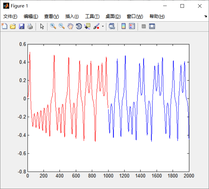
X_TR = X(1:n_tr);
X_TE = X(n_tr+1:n_tr+n_te);
figure,plot(1:1:n_tr,X_TR,'r');
hold on
plot(n_tr+1:1:n_tr+n_te,X_TE,'b');
hold off
 
[XN_TR,DN_TR] = PhaSpaRecon(X_TR,t,d);
[XN_TE,DN_TE] = PhaSpaRecon(X_TE,t,d);
 
%--------------------------------------------------------------------------
% Training and testing
 
P = XN_TR;
T = DN_TR;
spread = 1;       % The higher this value is,The value of the covered function is large(The default is 1)
net = newrbe(P,T,spread);
 
ERR1 = sim(net,XN_TR)-DN_TR;
err_mse1 = mean(ERR1.^2);
perr1 = err_mse1/var(X)
 
DN_PR = sim(net,XN_TE);
ERR2 = DN_PR-DN_TE;
err_mse2 = mean(ERR2.^2);
perr2 = err_mse2/var(X)
 
%--------------------------------------------------------------------------
% Result mapping
 
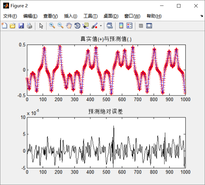
figure;
subplot(211);
plot(1:length(ERR2),DN_TE,'r+-',1:length(ERR2),DN_PR,'b-');
title('True value(+)And predicted value(.)')
subplot(212);
plot(ERR2,'k');
title('Prediction absolute error')
 

If you like, you can pay attention to me