1 particle swarm optimization

1.1 research background

The development process of particle swarm optimization algorithm. Particle swarm optimization algorithm (partial swarm optimization PSO), each particle in the particle swarm represents the possible solution of a problem. The intelligence of problem solving is realized through the simple behavior of the individual particle and the information interaction in the group. Due to its simple operation and fast convergence speed, PSO has been widely used in many fields such as function optimization, image processing, geodesy and so on With the expansion of application range, PSO algorithm has problems to be solved, such as premature convergence, dimension disaster and easy to fall into local extremum. There are mainly the following development directions.

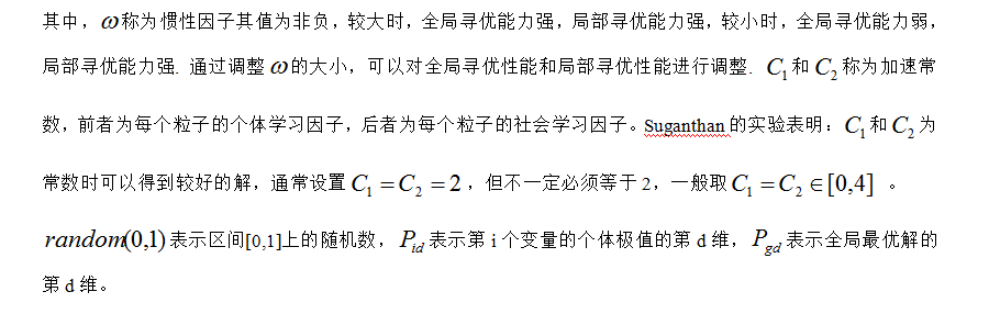
(1) Adjust the parameters of PSO to balance the global detection and local mining ability of the algorithm. For example, Shi and Eberhart introduce inertia weight into the velocity term of PSO algorithm, and linearly adjust the inertia weight according to the iterative process and particle flight (or nonlinear) dynamic adjustment to balance the globality and convergence speed of the search. In 2009, Zhang Wei and others studied the influence of acceleration factors on position expectation and variance based on the stability analysis of position expectation and variance of standard particle swarm optimization algorithm, and obtained a set of better acceleration factors.

(2) Design different types of topology and change the particle learning mode to improve the diversity of the population. Kennedy et al. Studied the impact of different topology on the performance of SPSO. In view of the shortcomings of easy premature convergence and low optimization accuracy of SPSO, a clearer form of particle swarm optimization algorithm: backbone particle swarm optimization algorithm was proposed in 2003 (Bare Bones PSO，BBPSO).

(3) Combining PSO with other optimization algorithms (or strategies) to form a hybrid PSO algorithm. For example, Zeng Yi embedded the pattern search algorithm into the PSO algorithm to realize the complementary advantages of the local search ability of the pattern search algorithm and the global optimization ability of the PSO algorithm.

(4) Niche technology is adopted. Niche is a bionic technology to simulate ecological balance, which is suitable for the optimization of multimodal function and multi-objective function. For example, in PSO algorithm, by constructing niche topology, the population is divided into several sub populations to dynamically form a relatively independent search space, so as to realize the synchronous search of multiple extreme regions, so as to avoid the algorithm Premature convergence occurs in solving multimodal function optimization problems. Parsopoulos proposes a multi population PSO algorithm based on the idea of "divide and conquer". Its core idea is to decompose the high-dimensional objective function into multiple low-dimensional functions, and then each low-dimensional sub function is optimized by a sub particle swarm optimization. This algorithm provides a better idea for solving high-dimensional problems.

Different development directions represent different application fields. Some need continuous global detection, some need to improve the optimization accuracy, some need the balance between global search and local search, and others need to solve high-dimensional problems. There is no comparability between the good and the bad in these directions, only the difference of choosing the most appropriate method for solving different problems in different fields.

1.2 relevant models and ideas

Particle swarm optimization Particle swarm optimization (PSO) was first proposed by Eberhart and Kennedy in 1995. Its basic concept comes from the research on the foraging behavior of birds. Imagine a scenario: a group of birds are randomly searching for food. There is only one piece of food in this area. All birds do not know where the food is, but they know how far away the current location is from the food. The simplest scenario is Single effective strategy? Look for the individual nearest to the food in the flock to search for elements. PSO algorithm is inspired by the behavior characteristics of biological population and used to solve optimization problems.

A particle is used to simulate the above bird individuals. Each particle can be regarded as a search individual in the N-dimensional search space, and the current position of the particle is a candidate solution to the corresponding optimization problem, The flight process of a particle is the search process of the individual. The flight speed of a particle can be dynamically adjusted according to the historical optimal position of the particle and the historical optimal position of the population. A particle has only two attributes: speed and position. Speed represents the speed of movement and position represents the direction of movement. The optimal solution searched by each particle individually is called individual extremum, and the optimal individual extremum in the particle swarm is the current global optimal solution. Continuously iterate and update speed and position. Finally, the optimal solution satisfying the termination condition is obtained.

The algorithm flow is as follows:

1. Initialization

Firstly, we set the maximum number of iterations, the number of independent variables of the objective function, the maximum speed of particles and the position information as the whole search space. We randomly initialize the speed and position in the speed interval and search space, set the particle swarm size to M, and each particle randomly initializes a flying speed.

2. Individual extremum and global optimal solution

The fitness function is defined. The individual extremum is the optimal solution found for each particle. Finding a global value from these optimal solutions is called this global optimal solution. Compare with the historical global optimum and update it.

3. Update formulas for speed and position

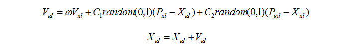
4. Termination conditions

(1) Reach the set number of iterations; (2) the difference between algebras meets the minimum limit

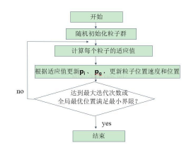
The above is the most basic standard PSO algorithm flow. Like other swarm intelligence algorithms, there is always a contradiction between the diversity of population and the convergence speed of PSO algorithm in the optimization process. The purpose of the improvement of standard PSO algorithm, whether the selection of parameters, the adoption of niche technology or the integration of other technologies with PSO, is to maintain the diversity of population while strengthening the local search ability of the algorithm, Prevent the algorithm from premature convergence while fast convergence.

2 Introduction to grid map

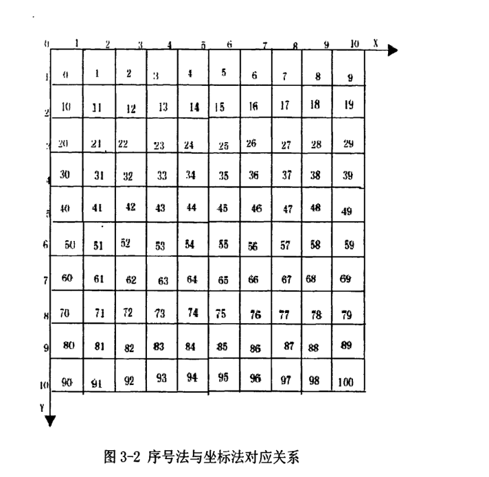
There are two methods to represent grid map, rectangular coordinate system method and sequence number method. Sequence number method saves memory than rectangular coordinate method

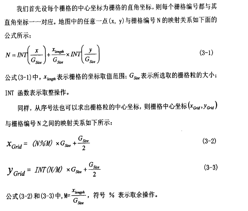
Modeling steps of indoor environment grid method

1. Selection of grid particle size

The size of the grid is a key factor. The selected grid is small, the environmental resolution is large, the storage of environmental information is large, and the decision-making speed is slow.

The grid selection is large, the environmental resolution is small, the storage of environmental information is small, and the decision-making speed is fast, but the ability to find paths in dense obstacle environment is weak.

2. Determination of obstacle grid

When the robot newly enters an environment, it does not know the information of indoor obstacles, which requires the robot to traverse the whole environment, detect the location of obstacles, find the serial number value in the corresponding grid map according to the location of obstacles, and modify the corresponding grid value. The free grid is assigned 0 to the grid without obstacles, and the obstacle grid is assigned 1 to the grid with obstacles

3. Establishment of grid map of unknown environment

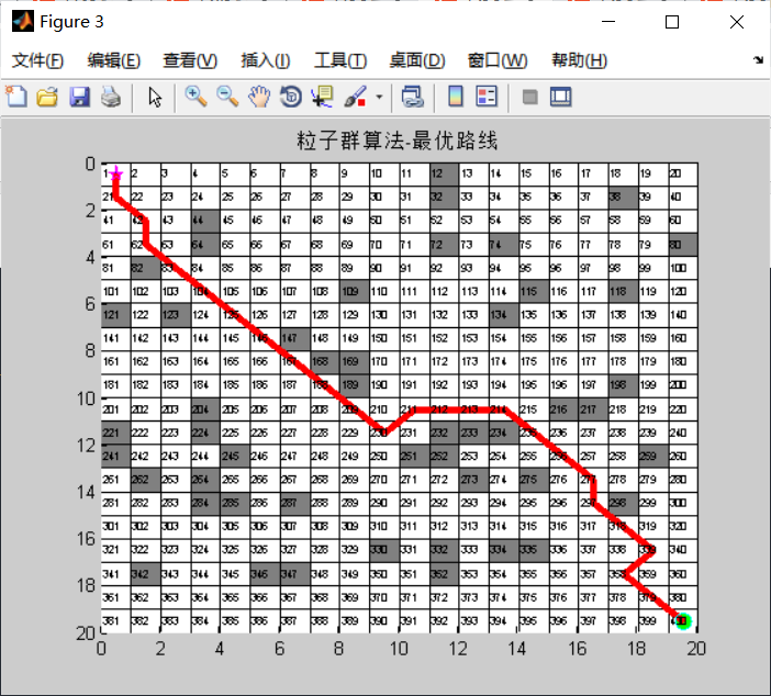
The end point is usually set as an unreachable point, For example (- 1, - 1), at the same time, the robot follows the principle of "lower right, upper left" in the process of path finding, that is, the robot walks downward first. When the robot encounters an obstacle in front, the robot turns to the right. Following this rule, the robot can finally search all feasible paths, and the robot will eventually return to the starting point.

Note: on the grid map, there is a principle that the size of obstacles is always equal to the size of n grids, and half a grid will not appear.

3 code

%% Particle swarm optimization
clc;
close all
clear
load('data4.mat')
figure(1)%Draw obstacle map
hold on
S=(S_coo(2)-0.5)*num_shange+(S_coo(1)+0.5);%Number corresponding to the starting point
E=(E_coo(2)-0.5)*num_shange+(E_coo(1)+0.5);%Number corresponding to the end point
for i=1:num_shange
    for j=1:num_shange
        if sign(i,j)==1
            y=[i-1,i-1,i,i];
            x=[j-1,j,j,j-1];
            h=fill(x,y,'k');
            set(h,'facealpha',0.5)
        end
        s=(num2str((i-1)*num_shange+j));
        %text(j-0.95,i-0.5,s,'fontsize',6)
    end
end
axis([0 num_shange 0 num_shange])%Boundary of restricted graph
plot(S_coo(2),S_coo(1), 'p','markersize', 10,'markerfacecolor','b','MarkerEdgeColor', 'm')%Draw starting point
plot(E_coo(2),E_coo(1),'o','markersize', 10,'markerfacecolor','g','MarkerEdgeColor', 'c')%Draw the end
set(gca,'YDir','reverse');%Image flip
for i=1:num_shange
    plot([0 num_shange],[i-1 i-1],'k-');
    plot([i i],[0 num_shange],'k-');%Draw grid lines
end
PopSize=20;%Population size
OldBestFitness=0;%Old optimal fitness value
gen=0;%Number of iterations
maxgen =100;%Maximum number of iterations
k1 = 1;%Crossover 1
k3 = 1;%Crossover 2
% c1=0.5;%Crossover probability
Pm=0.7;%Variation probability
c1=0.5;%Cognitive coefficient
c2=0.7;%Social learning coefficient
w=0.96;%Inertia coefficient
w_min=0.5;
w_max=1;
%%
%Initialization path


%Optimal solution
index1=find(best_route==E);
route_lin=best_route(1:index1);
for i=2:index1
    Q1=[mod(route_lin(i-1)-1,num_shange)+1-0.5,ceil(route_lin(i-1)/num_shange)-0.5];
    Q2=[mod(route_lin(i)-1,num_shange)+1-0.5,ceil(route_lin(i)/num_shange)-0.5];
    plot([Q1(1),Q2(1)],[Q1(2),Q2(2)],'r','LineWidth',3)
end
title('Particle swarm optimization-genetic algorithm-Comparison route');
figure(3)
hold on
for i=1:num_shange
    for j=1:num_shange
        if sign(i,j)==1
            y=[i-1,i-1,i,i];
            x=[j-1,j,j,j-1];
            h=fill(x,y,'k');
            set(h,'facealpha',0.5)
        end
        s=(num2str((i-1)*num_shange+j));
        text(j-0.95,i-0.5,s,'fontsize',6)
    end
end
axis([0 num_shange 0 num_shange])%Boundary of restricted graph
plot(S_coo(2),S_coo(1), 'p','markersize', 10,'markerfacecolor','b','MarkerEdgeColor', 'm')%Draw starting point
plot(E_coo(2),E_coo(1),'o','markersize', 10,'markerfacecolor','g','MarkerEdgeColor', 'c')%Draw the end
set(gca,'YDir','reverse');%Image flip
for i=1:num_shange
    plot([0 num_shange],[i-1 i-1],'k-');
    plot([i i],[0 num_shange],'k-');%Draw grid lines
end
for i=2:index1
    Q1=[mod(route_lin(i-1)-1,num_shange)+1-0.5,ceil(route_lin(i-1)/num_shange)-0.5];
    Q2=[mod(route_lin(i)-1,num_shange)+1-0.5,ceil(route_lin(i)/num_shange)-0.5];
    plot([Q1(1),Q2(1)],[Q1(2),Q2(2)],'r','LineWidth',3)
end
title('Particle swarm optimization-genetic algorithm-Optimal route');


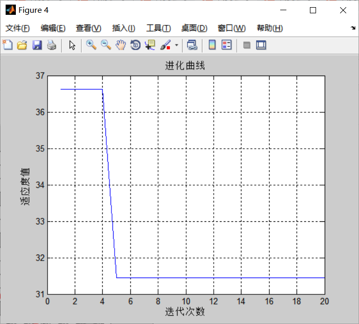
%Evolution curve
figure(4);
plot(BestFitness);
xlabel('Number of iterations')
ylabel('Fitness value')
grid on;
title('Particle swarm optimization-genetic algorithm-Evolution curve');
disp('Particle swarm optimization-genetic algorithm-Optimal route scheme:')
disp(num2str(route_lin))
disp(['Distance from start point to end point:',num2str(BestFitness(end))]);