I. concept of extreme learning machine
Extreme learning machine (ELM) is an algorithm for solving single hidden layer neural network proposed by Huang guangbin.
The biggest feature of ELM is that for traditional neural networks, especially single hidden layer feedforward neural networks (SLFNs), it is faster than traditional learning algorithms on the premise of ensuring learning accuracy.
2, Principle of limit learning machine
ELM is a new fast learning algorithm. For single hidden layer neural networks, ELM can randomly initialize the input weight and bias, and obtain the corresponding output weight.
(selected from Mr. Huang guangbin's PPT)
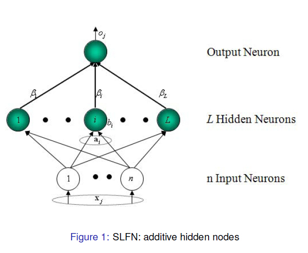
For a single hidden layer neural network (see Figure 1), it is assumed that An arbitrary sample
 , where
 ,
, . For a
 A single hidden layer neural network with multiple hidden layer nodes can be expressed as
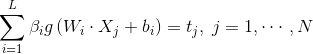
Among them, To activate the function,
 Enter a weight for,
 Is the output weight,
 Yes
Yes Offset of two hidden layer units.
 express
 and
and Inner product of.
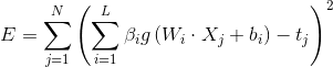
The goal of single hidden layer neural network learning is to minimize the output error, which can be expressed as
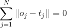
Namely existence ,
, and
and , so that
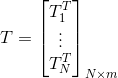
The matrix can be expressed as

Among them, Is the output of hidden layer nodes,
 Is the output weight,
 Is the desired output.

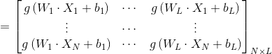
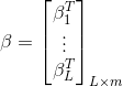 ,
,
In order to train single hidden layer neural networks, we hope to get ,
, and
and , so that
Among them, , this is equivalent to minimizing the loss function
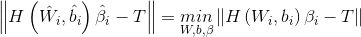
Some traditional algorithms based on gradient descent algorithm can be used to solve such problems, but the basic gradient based learning algorithm needs to adjust all parameters in the process of iteration. In ELM algorithm, once the weight is input And hidden layer offset
 The output matrix of the hidden layer is determined randomly
 Is uniquely identified. Training a single hidden layer neural network can be transformed into solving a linear system
 . And output weight
 Can be determined

Among them, It's a matrix
 Moore Penrose generalized inverse of. And the obtained solution can be proved
 The norm of is minimal and unique.
3, Particle swarm optimization
Particle swarm optimization algorithm was proposed by Dr. Eberhart and Dr. Kennedy in 1995. It comes from the study of bird predation behavior. Its basic core is to make use of the information sharing of individuals in the group, so as to make the movement of the whole group produce an evolutionary process from disorder to order in the problem-solving space, so as to obtain the optimal solution of the problem. Imagine this scenario: a flock of birds are foraging, and there is a corn field in the distance. All the birds don't know where the corn field is, but they know how far their current position is from the corn field. Then the best strategy to find the corn field, and the simplest and most effective strategy, is to search the surrounding area of the nearest bird group to the corn field.
In PSO, the solution of each optimization problem is a bird in the search space, which is called "particle", and the optimal solution of the problem corresponds to the "corn field" found in the bird swarm. All particles have a position vector (the position of the particle in the solution space) and a velocity vector (which determines the direction and speed of the next flight), and the fitness value of the current position can be calculated according to the objective function, which can be understood as the distance from the "corn field". In each iteration, the examples in the population can learn not only according to their own experience (historical position), but also according to the "experience" of the optimal particles in the population, so as to determine how to adjust and change the flight direction and speed in the next iteration. In this way, the whole population will gradually tend to the optimal solution.
The above explanation may be more abstract. Let's illustrate it with a simple example
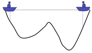
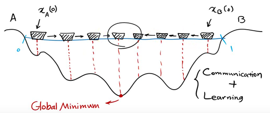
There are two people in a lake. They can communicate with each other and detect the lowest point of their position. The initial position is shown in the figure above. Because the right side is deep, the people on the left will move the boat to the right.
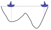
Now the left side is deep, so the person on the right will move the boat to the left
Keep repeating the process and the last two boats will meet
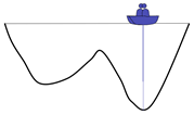
A local optimal solution is obtained
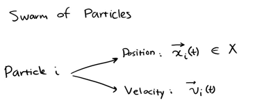
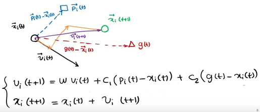
Represent each individual as a particle. The position of each individual at a certain time is expressed as x(t), and the direction is expressed as v(t)
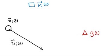
p (T) is the optimal solution of individual x at time t, g(t) is the optimal solution of all individuals at time t, v(t) is the direction of individual at time t, and x(t) is the position of individual at time t
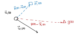
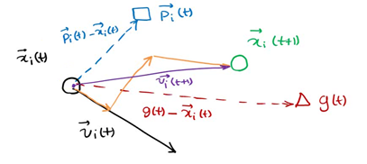
The next position is shown in the figure above, which is determined by X, P and G
The particles in the population can find the optimal solution of the problem by constantly learning from the historical information of themselves and the population.
However, in the follow-up research, the table shows that there is a problem in the above original formula: the update of V in the formula is too random, which makes the global optimization ability of the whole PSO algorithm strong, but the local search ability is poor. In fact, we need that PSO has strong global optimization ability in the early stage of algorithm iteration, and the whole population should have stronger local search ability in the later stage of algorithm iteration. Therefore, according to the above disadvantages, shi and Eberhart modified the formula by introducing inertia weight, so as to put forward the inertia weight model of PSO:
The components of each vector are represented as follows
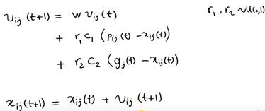
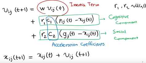
Where W is called the inertia weight of PSO, and its value is between [0,1]. Generally, adaptive value method is adopted, that is, w=0.9 at the beginning, which makes PSO have strong global optimization ability. With the deepening of iteration, the parameter W decreases, so that PSO has strong local optimization ability. When the iteration is over, w=0.1. The parameters c1 and c2 are called learning factors and are generally set to 14961; r1 and r2 are random probability values between [0,1].
The algorithm framework of the whole particle swarm optimization algorithm is as follows:
Step 1 population initialization can be carried out randomly or design a specific initialization method according to the optimized problem, and then calculate the individual fitness value, so as to select the individual local optimal position vector and the global optimal position vector of the population.
Step 2 iteration setting: set the number of iterations and set the current number of iterations to 1
step3 speed update: update the speed vector of each individual
step4 position update: update the position vector of each individual
Step 5 local position and global position vector update: update the local optimal solution of each individual and the global optimal solution of the population
Step 6 termination condition judgment: the maximum number of iterations is reached when judging the number of iterations. If it is satisfied, the global optimal solution is output. Otherwise, continue the iteration and jump to step 3.
For the application of particle swarm optimization algorithm, it is mainly the design of velocity and position vector iterative operators. Whether the iterative operator is effective or not will determine the performance of the whole PSO algorithm, so how to design the iterative operator of PSO is the research focus and difficulty in the application of PSO algorithm.
4, Demo code
clc;clear;close all;
%% Initialize population
N = 500;                         % Number of initial population
d = 24;                          % Spatial dimension
ger = 300;                      % Maximum number of iterations

          % Set position parameter limits(The form of matrix can be multidimensional)
vlimit = [-0.5, 0.5;-0.5, 0.5;-0.5, 0.5;-0.5, 0.5;-0.5, 0.5;-0.5, 0.5;
    -0.5, 0.5;-0.5, 0.5;-0.5, 0.5;-0.5, 0.5;-0.5, 0.5;-0.5, 0.5;
    -0.5, 0.5;-0.5, 0.5;-0.5, 0.5;-0.5, 0.5;-0.5, 0.5;-0.5, 0.5;
    -0.5, 0.5;-0.5, 0.5;-0.5, 0.5;-0.5, 0.5;-0.5, 0.5;-0.5, 0.5;];               % Set speed limit
c_1 = 0.8;                        % Inertia weight
c_2 = 0.5;                       % Self learning factor
c_3 = 0.5;                       % Group learning factor
 for i = 1:d
    x(:,i) = limit(i, 1) + (limit(i, 2) - limit(i, 1)) * rand(N, 1);%Location of initial population
end
v = 0.5*rand(N, d);                  % Speed of initial population
xm = x;                          % Historical best location for each individual
ym = zeros(1, d);                % Historical best position of population
fxm = 100000*ones(N, 1);               % Historical best fitness of each individual
fym = 10000;                      % Best fitness of population history
%% Particle swarm optimization
iter = 1;
times = 1;
record = zeros(ger, 1);          % Recorder
while iter <= ger
    for i=1:N
     fx(i) = calfit(x(i,:)) ; % Individual current fitness
    end
     for i = 1:N
        if fxm(i) > fx(i)
            fxm(i) = fx(i);     % Update the best fitness of individual history
            xm(i,:) = x(i,:);   % Update the best location in individual history
        end
     end
if fym > min(fxm)
        [fym, nmax] = min(fxm);   % Update group history best fit
        ym = xm(nmax, :);      % Update the best location in group history
 end
    v = v * c_1 + c_2 * rand *(xm - x) + c_3 * rand *(repmat(ym, N, 1) - x);% Speed update
    % Boundary velocity processing
    for i=1:d
        for j=1:N
        if  v(j,i)>vlimit(i,2)
            v(j,i)=vlimit(i,2);
        end
        if  v(j,i) < vlimit(i,1)
            v(j,i)=vlimit(i,1);
        end
        end
    end
    x = x + v;% Location update
    % Boundary location processing
    for i=1:d
        for j=1:N
        if  x(j,i)>limit(i,2)
            x(j,i)=limit(i,2);
        end
        if  x(j,i) < limit(i,1)
            x(j,i)=limit(i,1);
        end
        end
    end
    record(iter) = fym;%Maximum record
    iter = iter+1;
    times=times+1;
end
disp(['Minimum:',num2str(fym)]);
disp(['Variable value:',num2str(ym)]);
figure
plot(record)
xlabel('Number of iterations');
ylabel('Fitness value')
5, References
[1] You Lingling Research on limit learning machine based on particle swarm optimization algorithm and its application in precipitation prediction [D] Jilin Agricultural University, 2020