The selection of prediction model parameters plays an important role in its generalization ability and prediction accuracy. The parameters of least squares support vector machine based on RBF kernel function mainly involve penalty factor and kernel function parameters. The selection of these two parameters will directly affect the learning and generalization ability of least squares support vector machine. In order to improve the prediction results of least squares support vector machine, gray wolf optimization algorithm is used to optimize its parameters and establish software aging prediction model. Experiments show that the model has a good effect on the prediction of software aging.
The defects left in the software will cause computer memory leakage, rounding error accumulation, file lock not released and other phenomena with the long-term continuous operation of the software system, resulting in the decline or even collapse of the system performance. The occurrence of these software aging phenomena not only reduces the system reliability, but also endangers the safety of human life and property. In order to reduce the harm caused by software aging, it is particularly important to predict the software aging trend and adopt anti-aging strategies to avoid software aging [1].
Many scientific research institutions at home and abroad, such as Bell Labs, IBM, Nanjing University, Wuhan University [2], Xi'an Jiaotong University [3], have carried out in-depth research on software aging and achieved some results. Their main research direction is to find the best execution time of software anti-aging strategy by predicting the software aging trend.
This paper takes Tomcat server as the research object, monitors the operation of tomcat, collects system performance parameters, and establishes the least squares support vector machine software aging prediction model based on gray wolf optimization algorithm. Predict the software running state and determine the execution time of software anti-aging strategy.
Least squares support vector machine
Support Vector Machine (SVM) was proposed by Cortes and Vapnik[4]. Based on VC dimension theory and structural risk minimization principle, SVM can well solve the problems of small samples, nonlinearity, high dimension and local minimum.
When the number of training samples is more, the SVM is more complex to solve the quadratic programming problem, and the model training time is too long. Snykens et al. [5] proposed Least Squares Support Vector Machine (Least Squares Support Vector Machine, LSSVM), Gen P uses equality constraints instead of inequality constraints on the basis of SVM, and transforms the quadratic programming problem into a system of linear equations, which largely avoids a large number of complex calculations of SVM and reduces the difficulty of training. In recent years, LSSVM has been widely used in regression estimation, nonlinear modeling and other fields, and achieved good prediction effect.
In this paper, RBF kernel function is used as the kernel function of LSSVM model. The parameters of LSSVM algorithm based on RBF kernel function mainly involve penalty factor C and kernel function parameters ". In this paper, gray wolf optimization algorithm is used to optimize the parameters of LSSVM.
2 gray wolf optimization algorithm
In 2014, Mirjalili et al. [6] proposed grey wolf optimization (Grey WolfOptimizer, GWO) algorithm, GWO algorithm searches for the optimal value by simulating the hierarchy and predator-prey strategy of gray wolves in nature. GWO algorithm has attracted much attention because of its fast convergence and less adjustment parameters, and shows more advantages in solving function optimization problems. This method is superior to particle swarm optimization algorithm, differential evolution algorithm and citation algorithm in global search and convergence The force search algorithm is widely used in the fields of feature subset selection, surface wave parameter optimization and so on.
2.1 grey wolf optimization algorithm principle
Gray wolf individuals achieve the prosperity and development of the population through cooperation. Especially in the process of hunting, gray wolf group has a strict pyramid social hierarchy. The wolf with the highest level is α, The remaining gray wolf individuals were marked as β,δ,ω, They cooperate in predation.
In the whole gray wolf group, α Wolves play the role of leaders in the hunting process, responsible for decision-making in the hunting process and managing the whole wolf pack; β Wolf and δ Wolves are the second most adaptable group, and they help α Wolves manage the whole pack and have decision-making power in the process of hunting; The remaining gray wolf individuals are defined as ω, assist α,β,δ Attack prey.
2.2 description of grey wolf optimization algorithm
GWO algorithm imitates the hunting behavior of wolves and divides the whole hunting process into three stages: encirclement, pursuit and attack. The process of capturing prey is the process of finding the optimal solution. Assuming that the solution space of gray wolf is V-dimensional, gray wolf group x is composed of N gray wolf individuals, that is, X=[Xi; X2,..., XN]; For the gray wolf Xi (1 ≤ i ≤ n), its position Xi=[Xi1; Xi2,..., XiV] in the V-dimensional space. The distance between the gray wolf individual position and the prey position is measured by the fitness. The smaller the distance, the greater the fitness. The optimization process of GWO algorithm is as follows.
2.2. 1 surround
Firstly, the prey is surrounded. In this process, the distance between the prey and the gray wolf is expressed by a mathematical model as follows:
Where: Xp (m) is the prey position after the m-th iteration, X (m) is the gray wolf position, D is the distance between the gray wolf and the prey, A and C are the convergence factor and swing factor respectively, and the calculation formula is:
2.2. 2 pursuit
The optimization process of GWO algorithm is based on α,β and δ To locate the prey. ω Wolf in α,β,δ Under the guidance of the wolf, hunt the prey, update their respective positions according to the position of the current best search unit, and α,β,δ Position to reposition the prey. The individual position of wolves will change with the escape of prey. The mathematical description of the update process at this stage is as follows:
2.2. 3 attack
Wolves attack prey and capture prey to obtain the optimal solution. This process is realized by decreasing in equation (2). When 1 ≤∣ A ∣, it indicates that the wolf pack will be closer to the prey, then the wolf pack will narrow the search scope for local search; when 1 < ∣ A ∣, the wolf pack will disperse away from the prey, expand the search scope for global search
-
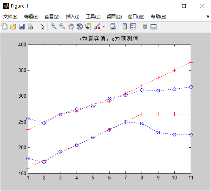
tic % time
%% Empty environment import data
clear
clc
close all
format long
load wndspd
%% GWO-SVR
input_train=[
    560.318,1710.53; 562.267,1595.17; 564.511,1479.78; 566.909,1363.74; 569.256,1247.72; 571.847,1131.3; 574.528,1015.33;
    673.834,1827.52; 678.13,1597.84; 680.534,1482.11; 683.001,1366.24; 685.534,1250.1; 688.026,1133.91; 690.841,1017.81;
    789.313,1830.18; 791.618,1715.56; 796.509,1484.76; 799.097,1368.85; 801.674,1252.76; 804.215,1136.49; 806.928,1020.41;
    904.711,1832.73; 907.196,1718.05; 909.807,1603.01; 915.127,1371.43; 917.75,1255.36; 920.417,1139.16; 923.149,1023.09;
    1020.18,1835.16; 1022.94,1720.67; 1025.63,1605.48; 1028.4,1489.91; 1033.81,1258.06; 1036.42,1141.89; 1039.11,1025.92;
    1135.36,1837.45; 1138.33,1722.94; 1141.35,1607.96; 1144.25,1492.43; 1147.03,1376.63; 1152.23,1144.56; 1154.83,1028.73;
    1250.31,1839.19; 1253.44,1725.01; 1256.74,1610.12; 1259.78,1494.74; 1262.67,1379.1; 1265.43,1263.29; 1270.48,1031.58;
    1364.32,1840.51; 1367.94,1726.52; 1371.2,1611.99; 1374.43,1496.85; 1377.53,1381.5; 1380.4,1265.81; 1382.89,1150.18;
    1477.65,1841.49; 1481.34,1727.86; 1485.07,1613.64; 1488.44,1498.81; 1491.57,1383.71; 1494.47,1268.49; 1497.11,1153.04;
    1590.49,1842.51; 1594.53,1729.18; 1598.15,1615.15; 1601.61,1500.72; 1604.72,1385.93; 1607.78,1271.04; 1610.43,1155.93;
    1702.82,1843.56; 1706.88,1730.52; 1710.65,1616.79; 1714.29,1502.66; 1717.69,1388.22; 1720.81,1273.68; 1723.77,1158.8;
    ];
input_test=[558.317,1825.04; 675.909,1712.89; 793.979,1600.35; 912.466,1487.32;
    1031.17,1374.03; 1149.79,1260.68; 1268.05,1147.33; 1385.36,1034.68;1499.33,1037.87;1613.11,1040.92;1726.27,1044.19;];

output_train=[
    235,175; 235,190; 235,205; 235,220; 235,235; 235,250; 235,265;
    250,160; 250,190; 250,205; 250,220; 250,235; 250,250; 250,265;
    265,160; 265,175; 265,205; 265,220; 265,235; 265,250; 265,265;
    270,160; 270,175; 270,190; 270,220; 270,235; 270,250; 270,265;
    285,160; 285,175; 285,190; 285,205; 285,235; 285,250; 285,265;
    290,160; 290,175; 290,190; 290,205; 290,220; 290,250; 290,265;
    305,160; 305,175; 305,190; 305,205; 305,220; 305,235; 305,265;
    320,160; 320,175; 320,190; 320,205; 320,220; 320,235; 320,250;
    335,160; 335,175; 335,190; 335,205; 335,220; 335,235; 335,250;
    350,160; 350,175; 350,190; 350,205; 350,220; 350,235; 350,250;
    365,160; 365,175; 365,190; 365,205; 365,220; 365,235; 365,250;

    ];
output_test=[235,160; 250,175; 265,190;270,205; 285,220; 290,235; 305,250; 320,265; 335,265; 350,265; 365,265;];

% Generate data to be regressed
x = [0.1,0.1;0.2,0.2;0.3,0.3;0.4,0.4;0.5,0.5;0.6,0.6;0.7,0.7;0.8,0.8;0.9,0.9;1,1];
y = [10,10;20,20;30,30;40,40;50,50;60,60;70,70;80,80;90,90;100,100];
X = input_train;
Y = output_train;
Xt = input_test;
Yt = output_test;
%% Using gray wolf algorithm to select the best SVR parameter
SearchAgents_no=60; % Number of wolves
Max_iteration=500; % Maximum number of iterations
dim=2; % This example needs to optimize two parameters c and g
lb=[0.1,0.1]; % Lower bound of parameter value
ub=[100,100]; % Upper bound of parameter value

Alpha_pos=zeros(1,dim); % initialization Alpha Wolf position
Alpha_score=inf; % initialization Alpha The objective function value of the wolf, change this to -inf for maximization problems

Beta_pos=zeros(1,dim); % initialization Beta Wolf position
Beta_score=inf; % initialization Beta The objective function value of the wolf, change this to -inf for maximization problems

Delta_pos=zeros(1,dim); % initialization Delta Wolf position
Delta_score=inf; % initialization Delta The objective function value of the wolf, change this to -inf for maximization problems

Positions=initialization(SearchAgents_no,dim,ub,lb);

Convergence_curve=zeros(1,Max_iteration);

l=0; % Cycle counter


% %% SVM Network regression prediction
% [output_test_pre,acc,~]=svmpredict(output_test',input_test',model_gwo_svr); % SVM Model prediction and its accuracy
% test_pre=mapminmax('reverse',output_test_pre',rule2);
% test_pre = test_pre';
%
% gam = [bestc bestc]; % Regularization parameter
% sig2 =[bestg bestg];
% model = initlssvm(X,Y,type,gam,sig2,kernel);                 % Model initialization
% model = trainlssvm(model);  % train
% Yp = simlssvm(model,Xt);    % regression

plot(1:length(Yt),Yt,'r+:',1:length(Yp),Yp,'bo:')
title('+Is the true value, o Is the predicted value')


% err_pre=wndspd(104:end)-test_pre;
% figure('Name','Test data residual diagram')
% set(gcf,'unit','centimeters','position',[0.5,5,30,5])
% plot(err_pre,'*-');
% figure('Name','original-Prediction chart')
% plot(test_pre,'*r-');hold on;plot(wndspd(104:end),'bo-');
% legend('forecast','original')
% set(gcf,'unit','centimeters','position',[0.5,13,30,5])
%
% result=[wndspd(104:end),test_pre]
%
% MAE=mymae(wndspd(104:end),test_pre)
% MSE=mymse(wndspd(104:end),test_pre)
% MAPE=mymape(wndspd(104:end),test_pre)
%% Show program run time
toc