1, Introduction
1 concept of particle swarm optimization
Particle swarm optimization (PSO) is an evolutionary computing technology, which originates from the research on the predation behavior of birds. The basic idea of particle swarm optimization algorithm is to find the optimal solution through the cooperation and information sharing among individuals in the population
The advantage of PSO is that it is simple and easy to implement, and there is no adjustment of many parameters. At present, it has been widely used in function optimization, neural network training, fuzzy system control and other application fields of genetic algorithm.
2 particle swarm optimization analysis
2.1 basic ideas
Particle swarm optimization algorithm designs a massless particle to simulate the birds in the bird swarm. The particle has only two attributes: speed and position. Speed represents the speed of movement and position represents the direction of movement. Each particle separately searches for the optimal solution in the search space, records it as the current individual extreme value, shares the individual extreme value with other particles in the whole particle swarm, and finds the optimal individual extreme value as the current global optimal solution of the whole particle swarm, All particles in the particle swarm adjust their speed and position according to the current individual extreme value found by themselves and the current global optimal solution shared by the whole particle swarm. The following dynamic diagram vividly shows the process of PSO algorithm: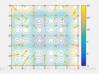
2 update rules
PSO is initialized as a group of random particles (random solutions). Then the optimal solution is found by iteration. In each iteration, the particles update themselves by tracking two "extreme values" (pbest, gbest). After finding these two optimal values, the particle updates its speed and position through the following formula.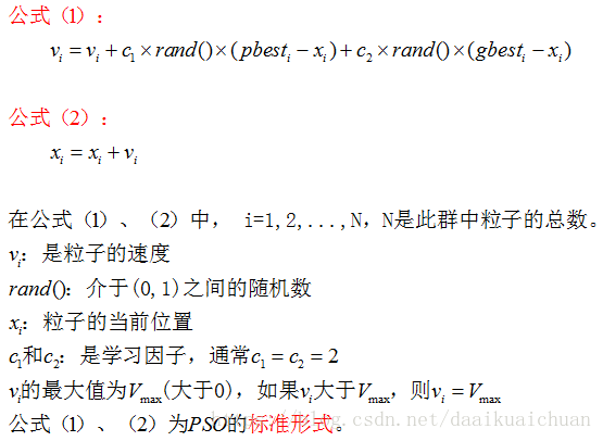
The first part of formula (1) is called [memory item], which indicates the influence of the last speed and direction; the second part of formula (1) is called [self cognition item], which is a vector from the current point to the best point of the particle itself, which indicates that the action of the particle comes from its own experience; the third part of formula (1) is called [group cognition item] is a vector from the current point to the best point of the population, which reflects the cooperation and knowledge sharing among particles. Particles determine the next movement through their own experience and the best experience of their peers. Based on the above two formulas, it forms the standard form of PSO.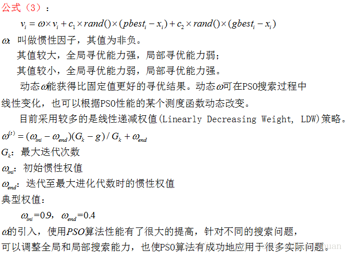
Equations (2) and (3) are considered as standard PSO algorithms.
3 PSO algorithm flow and pseudo code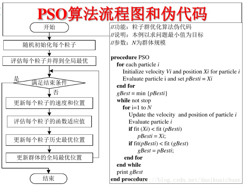
2, Partial code
function [L_best,xx,tourGbest]=main(data)

%% Download data
% data=load('coor.txt');
% cityCoor=data;%City coordinate matrix
cityCoor=data;


%% Calculate the distance between cities
n=size(cityCoor,1);            %Number of cities
cityDist=zeros(n,n);           %City distance matrix
for i=1:n
    for j=1:n
        if i~=j
            cityDist(i,j)=((cityCoor(i,1)-cityCoor(j,1))^2+...
                (cityCoor(i,2)-cityCoor(j,2))^2+(cityCoor(i,3)-cityCoor(j,3))^2)^0.5;
        end
        cityDist(j,i)=cityDist(i,j);
    end
end
nMax=10;                      %Evolution times
indiNumber=400;               %Number of individuals
individual=zeros(indiNumber,n);
%^Initialize particle position
for i=1:indiNumber
    individual(i,:)=randperm(n);
end

%% Calculate population fitness
indiFit=fitness(individual,cityDist);
[value,index]=min(indiFit);
tourPbest=individual;                              %Current individual optimal
tourGbest=individual(index,:) ;                    %Current global optimum
recordPbest=inf*ones(1,indiNumber);                %Individual optimal record
recordGbest=indiFit(index);                        %Group optimal record
xnew1=individual;

%% Loop to find the optimal path
L_best=zeros(1,nMax);
for N=1:nMax
N
    %Calculate fitness value
    indiFit=fitness(individual,cityDist);
%     %% Elite replication
%     [bad good order]=elite(individual,cityCoor,cityDist,0.1);  %Extract 10%Elite particle
%     elitenum=size(bad,2);
%     individual(bad,:)=individual(good,:);
     %% Elite replication learning
    [bad good order]=elite(individual,cityCoor,cityDist,0.1);  %Extract 10%Elite particle
    elitenum=size(bad,2);
    %Random adjustment
    for i=1:elitenum
%         better(i,:)=tsp(cityCoor,n,cityDist);
         better(i,:)=goodchange(individual(good(i),:),cityDist);
    end
    individual(bad,:)=better;


    %Update current best and historical best
    for i=1:indiNumber
        if indiFit(i)<recordPbest(i)
            recordPbest(i)=indiFit(i);
            tourPbest(i,:)=individual(i,:);
        end
        if indiFit(i)<recordGbest
            recordGbest=indiFit(i);
            tourGbest=individual(i,:);
        end
    end

    [value,index]=min(recordPbest);
    recordGbest(N)=recordPbest(index);

    %% Cross operation
    for i=1:indiNumber
       % Cross with individual optimal
        c1=unidrnd(n-1); %Generate cross bit
        c2=unidrnd(n-1); %Generate cross bit
        while c1==c2
            c1=round(rand*(n-2))+1;
            c2=round(rand*(n-2))+1;
        end
        chb1=min(c1,c2);
        chb2=max(c1,c2);
        cros=tourPbest(i,chb1:chb2);
        ncros=size(cros,2);
        %Delete the same element as the crossing area
        for j=1:ncros
            for k=1:n
                if xnew1(i,k)==cros(j)
                    xnew1(i,k)=0;
                    for t=1:n-k
                        temp=xnew1(i,k+t-1);
                        xnew1(i,k+t-1)=xnew1(i,k+t);
                        xnew1(i,k+t)=temp;
                    end
                end
            end
        end
        %Insert cross region
        xnew1(i,n-ncros+1:n)=cros;
        %Accept if the new path length becomes shorter
        dist=0;
        for j=1:n-1
            dist=dist+cityDist(xnew1(i,j),xnew1(i,j+1));
        end
        dist=dist+cityDist(xnew1(i,1),xnew1(i,n));
        if indiFit(i)>dist
            individual(i,:)=xnew1(i,:);
        end

        % Cross with all the best
        c1=round(rand*(n-2))+1;  %Generate cross bit
        c2=round(rand*(n-2))+1;  %Generate cross bit
        while c1==c2
            c1=round(rand*(n-2))+1;
            c2=round(rand*(n-2))+1;
        end
        chb1=min(c1,c2);
        chb2=max(c1,c2);
        cros=tourGbest(chb1:chb2);
        ncros=size(cros,2);
        %Delete the same element as the crossing area
        for j=1:ncros
            for k=1:n
                if xnew1(i,k)==cros(j)
                    xnew1(i,k)=0;
                    for t=1:n-k
                        temp=xnew1(i,k+t-1);
                        xnew1(i,k+t-1)=xnew1(i,k+t);
                        xnew1(i,k+t)=temp;
                    end
                end
            end
        end
        %Insert cross region
        xnew1(i,n-ncros+1:n)=cros;
        %Accept if the new path length becomes shorter
        dist=0;
        for j=1:n-1
            dist=dist+cityDist(xnew1(i,j),xnew1(i,j+1));
        end
        function path = tsp(loc,NumCity,distance)


% NumCity = length(loc); %Number of cities
% distance = zeros(NumCity); %Initialize distance matrix, 30 rows and 30 columns
%
% %Filling distance matrix
% for i = 1:NumCity,
%   for j = 1:NumCity,
%     %city i And cities j The distance between two points is the second-order norm between two points
%     distance(i, j) = norm(loc(i, :) - loc(j, :));
%   end
% end
%
% %The energy value is generated from the path through the objective function, which is the sum of the distances between cities
% %path = randperm(NumCity);
% %energy = sum(distance((path-1)*NumCity + [path(2:NumCity) path(1)]));

count = 1000;
all_dE = zeros(count, 1);

for i = 1:count
    path = randperm(NumCity); %Generate a path randomly, and the number is within 30

    %The distance is defined as the energy value, and the distance between all cities is added
    energy = sum(distance((path-1)*NumCity + [path(2:NumCity) path(1)]));
    new_path = path;
    index = round(rand(2,1)*NumCity+.5);
    inversion_index = (min(index):max(index));
    new_path(inversion_index) = fliplr(path(inversion_index));

    all_dE(i) = abs(energy - ...
    sum(sum(diff(loc([new_path new_path(1)],:))'.^2)));

end

dE = max(all_dE);%Record the maximum of 20 groups of energy difference
dE = max(all_dE);
temp = 10*dE; %Select a maximum difference as the starting temperature value

MaxTrialN = NumCity*100; % The maximum test temperature value is the maximum number of test solutions
MaxAcceptN = NumCity*10; % The maximum acceptable temperature value is the maximum number of acceptable solutions
StopTolerance = 0.005; %Tolerance, i.e. termination temperature value
StopTolerance = 0.005;
TempRatio = 0.4; %Temperature drop rate
minE = inf; %Initialize minimum energy value
maxE = -1; %Initialize maximum energy value
3, Operation results
