I. Introduction to BP neural network prediction algorithm
Note: Section 1.1 is mainly to summarize and help understand the principle of BP neural network algorithm considering influencing factors, that is, the explanation of conventional BP model training principle (whether to skip according to their own knowledge). Section 1.2 begins with the BP neural network prediction model based on the influence of historical values.
When BP neural network is used for prediction, there are mainly two types of models from the perspective of input indicators:
1.1 principle of BP neural network algorithm affected by relevant indexes
As shown in Figure 1, when training BP using MATLAB's newff function, it can be seen that most cases are three-layer neural networks (i.e. input layer, hidden layer and output layer). Here to help understand the principle of neural network:
1) Input layer: equivalent to human facial features. The facial features obtain external information and receive input data corresponding to the input port of neural network model.
2) hidden Layer: corresponding to the human brain, the brain analyzes and thinks about the data transmitted from the five senses. The hidden Layer of neural network maps the data X transmitted from the input layer, which is simply understood as a formula hidden Layer_ output=F(w*x+b). Among them, W and B are called weight and threshold parameters, and F() is the mapping rule, also known as the activation function, hiddenLayer_output is the output value of the hidden Layer for the transmitted data mapping. In other words, the hidden Layer maps the input influencing factor data X and generates the mapping value.
3) Output layer: it can correspond to human limbs. After thinking about the information from the five senses (hidden layer mapping), the brain controls the limbs to perform actions (respond to the outside). Similarly, the output layer of BP neural network is hidden layer_ Output is mapped again, outputLayer_output=w *hiddenLayer_output+b. Where W and B are weight and threshold parameters, and outputLayer_output is the output value (also called simulation value and prediction value) of the output layer of the neural network (understood as the external executive action of the human brain, such as the baby slapping the table).
4) Gradient descent algorithm: by calculating outputlayer_ For the deviation between output and the y value input by the neural network model, the algorithm is used to adjust the weight, threshold and other parameters accordingly. This process can be understood as that the baby beats the table and deviates. Adjust the body according to the distance of deviation, so that the arm waved again keeps approaching the table and finally hits the target.
Take another example to deepen understanding:
The BP neural network shown in Figure 1 has input layer, hidden layer and output layer. How does BP realize the output value outputlayer of the output layer through these three-layer structures_ Output, constantly approaching the given y value, so as to train to obtain an accurate model?
From the serial ports in the figure, we can think of a process: take the subway and imagine Figure 1 as a subway line. One day when Wang went home by subway: he got on the bus at the input starting station, passed many hiddenlayers on the way, and then found that he sat too far (the outputLayer corresponds to the current position), so Wang will be based on the distance from home (Error) according to the current position, Return to the midway subway station (hidden layer) and take the subway again (Error reverse transfer, using gradient descent algorithm to update w and b). If Wang makes another mistake, the adjustment process will be carried out again.
From the example of baby slapping the table and Wang taking the subway, think about the problem: for the complete training of BP, the data needs to be input first, and then through the mapping of the hidden layer, the BP simulation value is obtained from the output layer, and the parameters are adjusted according to the error between the simulation value and the Target value to make the simulation value approach the Target value continuously. For example, (1) the baby responds to external interference factors (x), and the brain constantly adjusts the position of the arms and controls the accuracy of the limbs (y, Target). (2) Wang Moumou goes to the boarding point (x), crosses the station (predict), and constantly returns to the midway station to adjust the position and get home (y, Target).
In these links, the influencing factor data x and the Target value data y (Target) are involved. According to x and y, BP algorithm is used to find the law between x and y, and realize the mapping and approximation of Y by x, which is the function of BP neural network algorithm. To add another word, the above processes are all BP model training. Although the training of the final model is accurate, is the bp network accurate and reliable. Therefore, we put x1 into the trained bp network to obtain the corresponding BP output value (predicted value) predict1. By mapping, calculating Mse, Mape, R and other indicators to compare the proximity of predict1 and y1, we can know whether the model is accurate or not. This is the test process of BP model, that is to realize the prediction of data, and compare the actual value to test whether the prediction is accurate.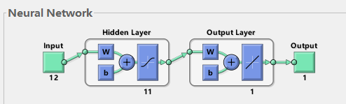
Fig. 1 3-layer BP neural network structure
1.2 BP neural network based on the influence of historical value
Taking the power load forecasting problem as an example, the two models are distinguished. When forecasting the power load in a certain period of time:
One way is to predict the load value at , t , time by considering the climate factor indicators at , t , time, such as the influence of air humidity x1, temperature x2 and holidays x3 at that time. This is the model mentioned in 1.1 above.
Another approach is to consider that the change of power load value is related to time. For example, it is considered that the power load value at time T-1, t-2 and t-3 is related to the load value at time t, that is, it satisfies the formula y(t)=F(y(t-1),y(t-2),y(t-3)). When BP neural network is used to train the model, the influencing factor values input to the neural network are historical load values y(t-1),y(t-2),y(t-3). In particular, 3 is called autoregressive order or delay. The output of y to the neural network is the value of T.
II. Whale algorithm
1. Enlighten
Whale optimization algorithm (WOA) is a new swarm intelligence optimization algorithm proposed by Mirjalili of Griffith University in Australia in 2016. Its advantages are simple operation, few parameters and strong ability to jump out of local optimization. 
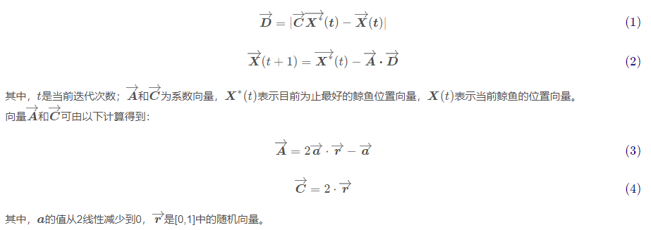
2. Surround prey
Humpback whales can recognize the location of their prey and turn around them. Because the position of the optimal position in the search space is unknown, WOA algorithm assumes that the current optimal candidate solution is the target prey or near the optimal solution. After the best candidate solution is defined, other candidate positions will try to move to the best position and update their positions. This behavior is represented by the following equation:

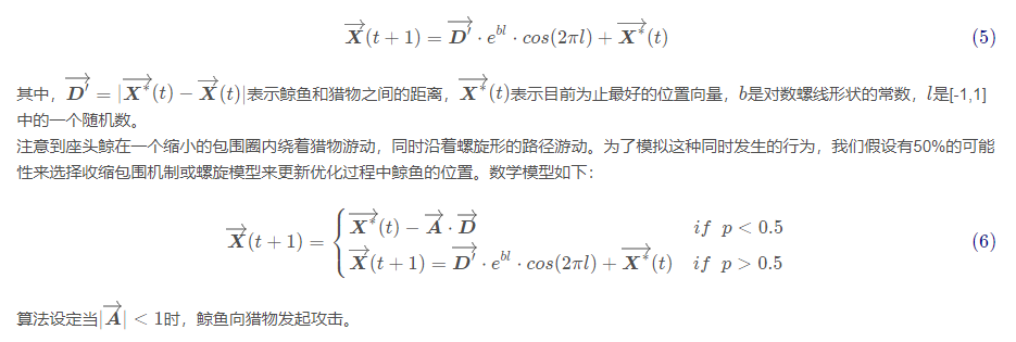
3. Hunting behavior
According to the hunting behavior of humpback whale, it swims to its prey in a spiral motion, so the mathematical model of hunting behavior is as follows:

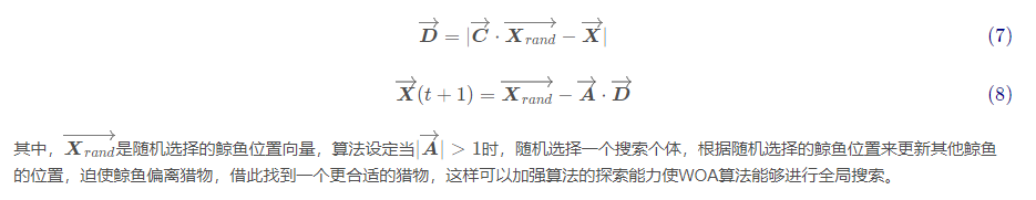
4. Search for prey
The mathematical model is as follows:

3, Steps of WOA Optimizing BP neural network
Step 1: initialize the weight and threshold of BP neural network
Step 2: calculate the length of decision variables of whale optimization algorithm and select the mean square error as the objective function of optimization.
Step 3: set the algorithm stop criteria, and use the genetic optimization algorithm to optimize the weights and threshold parameters of the neural network.
Step4: assign the optimized weight and threshold parameters to BP neural network.
Step 5: the optimized BP neural network is trained and tested, and the error analysis and accuracy comparison are carried out with the optimized BP neural network.
3, Demo code
%__________________________________________
% fobj = @YourCostFunction
% dim = number of your variables
% Max_iteration = maximum number of generations
% SearchAgents_no = number of search agents
% lb=[lb1,lb2,...,lbn] where lbn is the lower bound of variable n
% ub=[ub1,ub2,...,ubn] where ubn is the upper bound of variable n
% If all the variables have equal lower bound you can just
% define lb and ub as two single number numbers

% To run ALO: [Best_score,Best_pos,cg_curve]=ALO(SearchAgents_no,Max_iteration,lb,ub,dim,fobj)

% The Whale Optimization Algorithm
function [Leader_score,Leader_pos,Convergence_curve]=WOA(SearchAgents_no,Max_iter,lb,ub,dim,fobj,handles,value)

% initialize position vector and score for the leader
Leader_pos=zeros(1,dim);
Leader_score=inf; %change this to -inf for maximization problems


%Initialize the positions of search agents
Positions=initialization(SearchAgents_no,dim,ub,lb);

Convergence_curve=zeros(1,Max_iter);

t=0;% Loop counter

% Main loop
while t<Max_iter
    for i=1:size(Positions,1)

        % Return back the search agents that go beyond the boundaries of the search space
        Flag4ub=Positions(i,:)>ub;
        Flag4lb=Positions(i,:)<lb;
        Positions(i,:)=(Positions(i,:).*(~(Flag4ub+Flag4lb)))+ub.*Flag4ub+lb.*Flag4lb;

        % Calculate objective function for each search agent
        fitness=fobj(Positions(i,:));
        All_fitness(1,i)=fitness;

        % Update the leader
        if fitness<Leader_score % Change this to > for maximization problem
            Leader_score=fitness; % Update alpha
            Leader_pos=Positions(i,:);
        end

    end

    a=2-t*((2)/Max_iter); % a decreases linearly fron 2 to 0 in Eq. (2.3)

    % a2 linearly dicreases from -1 to -2 to calculate t in Eq. (3.12)
    a2=-1+t*((-1)/Max_iter);

    % Update the Position of search agents
    for i=1:size(Positions,1)
        r1=rand(); % r1 is a random number in [0,1]
        r2=rand(); % r2 is a random number in [0,1]

        A=2*a*r1-a;  % Eq. (2.3) in the paper
        C=2*r2;      % Eq. (2.4) in the paper


        b=1;               %  parameters in Eq. (2.5)
        l=(a2-1)*rand+1;   %  parameters in Eq. (2.5)

        p = rand();        % p in Eq. (2.6)

        for j=1:size(Positions,2)

            if p<0.5
                if abs(A)>=1
                    rand_leader_index = floor(SearchAgents_no*rand()+1);
                    X_rand = Positions(rand_leader_index, :);
                    D_X_rand=abs(C*X_rand(j)-Positions(i,j)); % Eq. (2.7)
                    Positions(i,j)=X_rand(j)-A*D_X_rand;      % Eq. (2.8)

                elseif abs(A)<1
                    D_Leader=abs(C*Leader_pos(j)-Positions(i,j)); % Eq. (2.1)
                    Positions(i,j)=Leader_pos(j)-A*D_Leader;      % Eq. (2.2)
                end

            elseif p>=0.5

                distance2Leader=abs(Leader_pos(j)-Positions(i,j));
                % Eq. (2.5)
                Positions(i,j)=distance2Leader*exp(b.*l).*cos(l.*2*pi)+Leader_pos(j);

            end

        end
    end

    t=t+1;
    Convergence_curve(t)=Leader_score;

    if t>2
        line([t-1 t], [Convergence_curve(t-1) Convergence_curve(t)],'Color','b')
        xlabel('Iteration');
        ylabel('Best score obtained so far');
        drawnow
    end


    set(handles.itertext,'String', ['The current iteration is ', num2str(t)])
    set(handles.optimumtext,'String', ['The current optimal value is ', num2str(Leader_score)])
    if value==1
        hold on
        scatter(t*ones(1,SearchAgents_no),All_fitness,'.','k')
    end


end
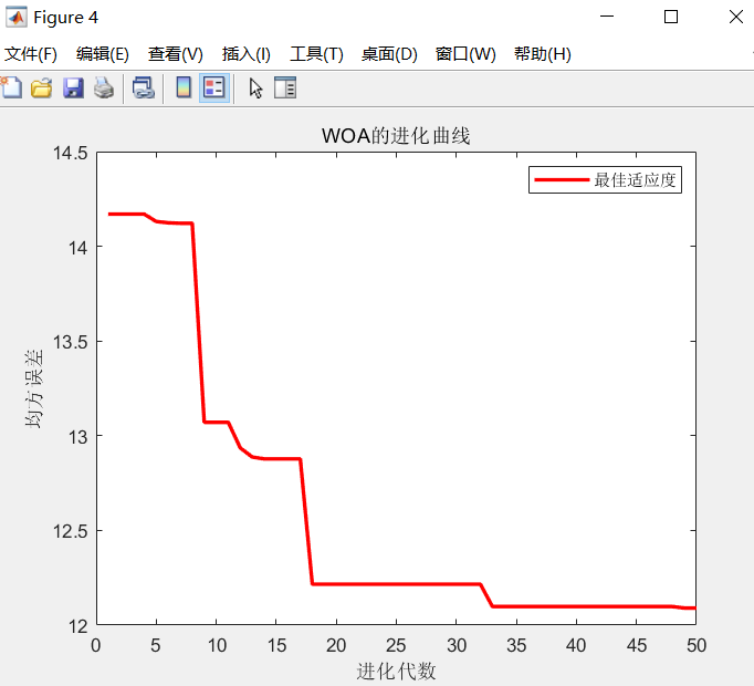
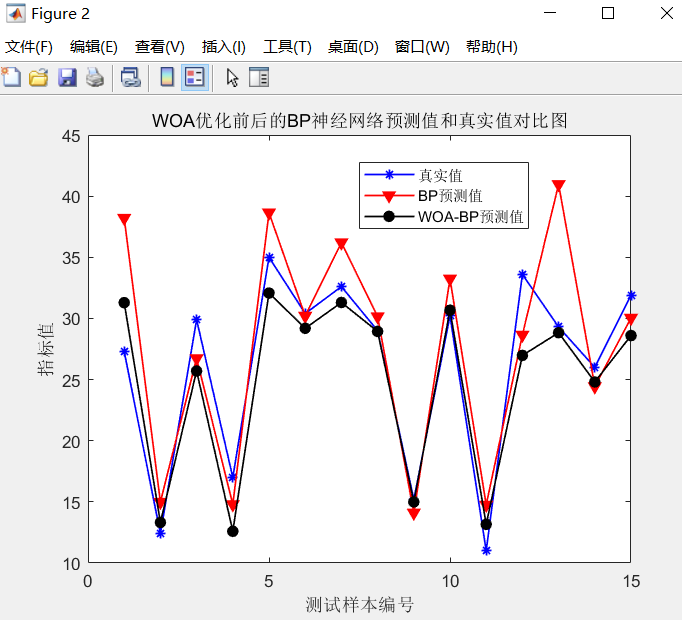
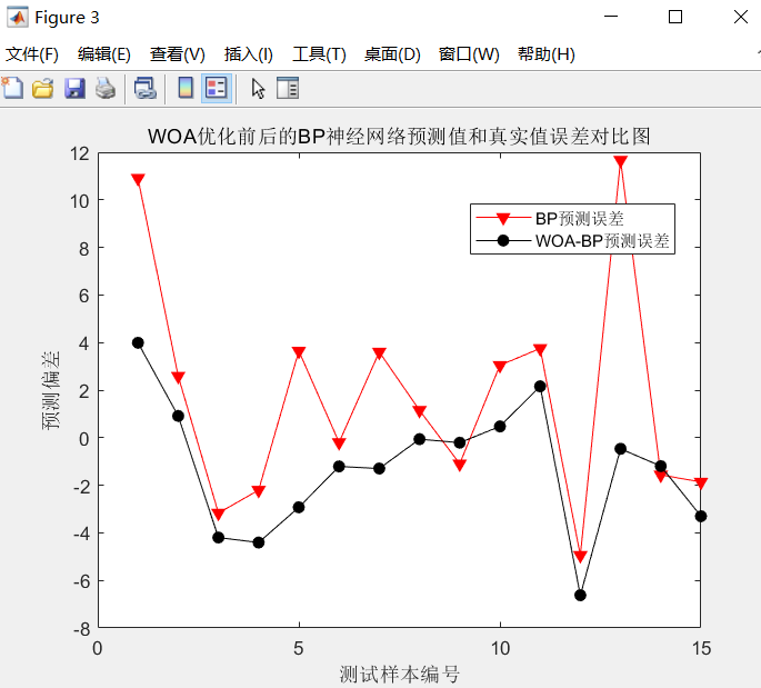
4, Simulation results
5, References
Prediction of water resources demand in Ningxia Based on BP neural network