1, Introduction
Mathematical morphology operations can be divided into binary morphology and gray morphology. Gray morphology is extended from binary morphology. Mathematical morphology has two basic operations, namely corrosion and expansion, and corrosion and expansion form open operation and closed operation through combination.
The open operation is to corrode and then expand, and the closed operation is to expand and then corrode.
1 binary morphology
Roughly speaking, corrosion can "reduce" the range of the target area, which essentially shrinks the boundary of the image and can be used to eliminate small and meaningless targets. The formula is expressed as:
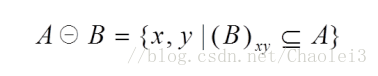
This formula indicates that structure B is used to corrode A. it should be noted that an origin needs to be defined in B, [and the moving process of B is consistent with the moving process of convolution kernel, which is the same as the calculation after the convolution kernel overlaps with the image] when the origin of B is translated to the pixel (x,y) of image a, if B is at (x,y), it is completely included in the overlapping area of image a, (that is, all the image values of a corresponding to the element position of 1 in B are also 1) assign the pixel (x,y) corresponding to the output image to 1, otherwise assign it to 0.
Let's look at a demo.
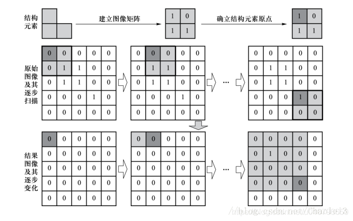
B moves on A in order (the same as the convolution kernel moves on the image, and then performs morphological operation on the coverage area of B). When the area covering A is [1,1; 1,1] or [1,0; 1,1] (that is, '1' in B is A subset of the coverage area), the position of the corresponding output image will be 1.
2 expansion
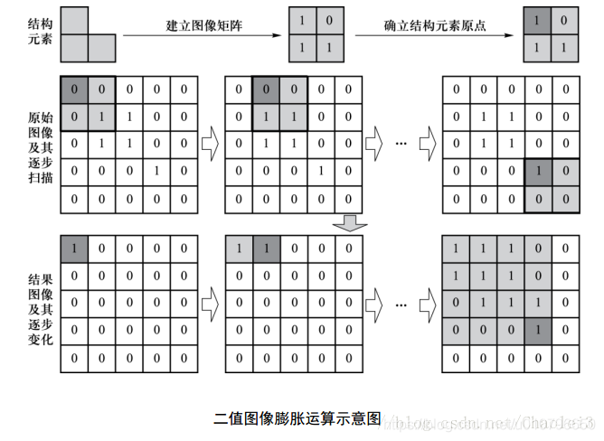
Roughly speaking, the expansion will "enlarge" the range of the target area, merge the background points in contact with the target area into the target object, and expand the target boundary to the outside. It can be used to fill some holes in the target area and eliminate the small particle noise contained in the target area.
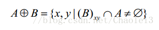
This formula represents expanding A with structure B and translating the origin of structure element B to the position of image pixel (x,y). If the intersection of B and A at the image pixel (x,y) is not empty (that is, at least one image value corresponding to A at the element position of 1 in B is 1), the pixel (x,y) corresponding to the output image is assigned as 1, otherwise it is assigned as 0.
The illustration is:
3 Summary
In other words, regardless of corrosion or expansion, the structural element B is translated on the image like a convolution operation. The origin in the structural element B is equivalent to the core center of the convolution core, and the result is also stored on the element corresponding to the core center. However, corrosion is that B is completely contained in the area covered by it, and B can intersect with the area covered by it during expansion.
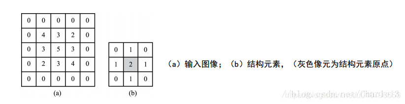
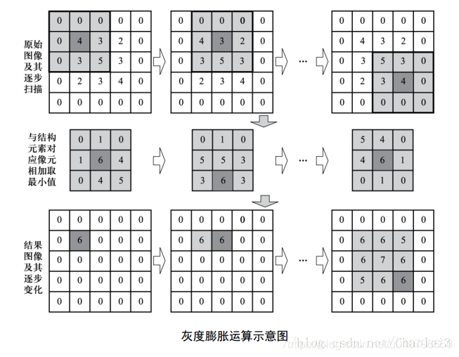
4 gray morphology
Before describing the gray value morphology, we make A convention that the area of image A covered by structural element B is marked as P (meaning Part).
5 corrosion of gray morphology
Then, corrosion in gray morphology is an operation similar to convolution. Use P to subtract the small rectangle formed by structural element B, and take the minimum value to assign it to the position of the corresponding origin.
Let's take a look at an example to deepen our understanding of gray morphology.
Suppose we have the following image A and structural element B:
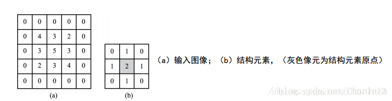
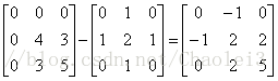
The process of gray morphology corrosion is as follows:
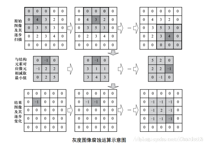
We show the output result of the first element of the output image, that is, the position of 4 corresponding to the origin. The values of other elements of the output image are also obtained in this way. We will see that the area covered by B is the subtracted matrix, and then find min (minimum value) in its difference matrix as the value of the corresponding position of the origin.
Expansion of gray morphology
According to the above description of corrosion, we make the same description of expansion. Expansion in gray morphology is an operation similar to convolution. Add P and B, and then assign the maximum value in this region to the position corresponding to the origin of structural element B.
Here is also a description of the origin of the first element value of the output image.

The maximum value of the sum of the above matrix is 6, so 6 is assigned to the position corresponding to the origin of the structural element.
6 Summary
The concept of gray morphology is introduced above. Here we will talk about their respective uses. Compared with the original image, each pixel becomes smaller as a result of corrosion, so it is suitable for removing peak noise. The result of gray value expansion will make each pixel larger than before, so it is suitable for removing Valley noise.
2, Source code
function varargout = untitled(varargin)
% UNTITLED M-file for untitled.fig
% UNTITLED, by itself, creates a new UNTITLED or raises the existing
% singleton*.
%
% H = UNTITLED returns the handle to a new UNTITLED or the handle to
% the existing singleton*.
%
% UNTITLED('CALLBACK',hObject,eventData,handles,...) calls the local
% function named CALLBACK in UNTITLED.M with the given input arguments.
%
% UNTITLED('Property','Value',...) creates a new UNTITLED or raises the
% existing singleton*. Starting from the left, property value pairs are
% applied to the GUI before untitled_OpeningFcn gets called. An
% unrecognized property name or invalid value makes property application
% stop. All inputs are passed to untitled_OpeningFcn via varargin.
%
% *See GUI Options on GUIDE's Tools menu. Choose "GUI allows only one
% instance to run (singleton)".
%
% See also: GUIDE, GUIDATA, GUIHANDLES
% Edit the above text to modify the response to help untitled
% Last Modified by GUIDE v2.5 21-May-2021 23:07:23
% Begin initialization code - DO NOT EDIT
gui_Singleton = 1;
gui_State = struct('gui_Name', mfilename, ...
'gui_Singleton', gui_Singleton, ...
'gui_OpeningFcn', @untitled_OpeningFcn, ...
'gui_OutputFcn', @untitled_OutputFcn, ...
'gui_LayoutFcn', [] , ...
'gui_Callback', []);
if nargin && ischar(varargin{1})
gui_State.gui_Callback = str2func(varargin{1});
end
if nargout
[varargout{1:nargout}] = gui_mainfcn(gui_State, varargin{:});
else
gui_mainfcn(gui_State, varargin{:});
end
% End initialization code - DO NOT EDIT
% --- Executes just before untitled is made visible.
function untitled_OpeningFcn(hObject, eventdata, handles, varargin)
% This function has no output args, see OutputFcn.
% hObject handle to figure
% eventdata reserved - to be defined in a future version of MATLAB
% handles structure with handles and user data (see GUIDATA)
% varargin command line arguments to untitled (see VARARGIN)
% Choose default command line output for untitled
handles.output = hObject;
% Update handles structure
guidata(hObject, handles);
% UIWAIT makes untitled wait for user response (see UIRESUME)
% uiwait(handles.figure1);
% --- Outputs from this function are returned to the command line.
function varargout = untitled_OutputFcn(hObject, eventdata, handles)
% varargout cell array for returning output args (see VARARGOUT);
% hObject handle to figure
% eventdata reserved - to be defined in a future version of MATLAB
% handles structure with handles and user data (see GUIDATA)
% Get default command line output from handles structure
varargout{1} = handles.output;
% --- Executes on button press in pushbutton1.
function pushbutton1_Callback(hObject, eventdata, handles)
% hObject handle to pushbutton1 (see GCBO)
% eventdata reserved - to be defined in a future version of MATLAB
% handles structure with handles and user data (see GUIDATA)
global im;
global str;
[filename,pathname]=uigetfile_new({'*.*'},'Select training picture...');
str=[pathname filename];
im=imread(str);
axes(handles.axes1);
imshow(im);
% --- Executes on button press in pushbutton2.
function pushbutton2_Callback(hObject, eventdata, handles)
% hObject handle to pushbutton2 (see GCBO)
% eventdata reserved - to be defined in a future version of MATLAB
% handles structure with handles and user data (see GUIDATA)
global im1;
global str1;
[filename,pathname]=uigetfile_new({'*.*'},'Select test picture...');
str1=[pathname filename];
im1=imread(str1);
axes(handles.axes2);
imshow(im1);
% --- Executes on button press in pushbutton3.
function pushbutton3_Callback(hObject, eventdata, handles)
% hObject handle to pushbutton3 (see GCBO)
% eventdata reserved - to be defined in a future version of MATLAB
% handles structure with handles and user data (see GUIDATA)
global im;
global im1;
global str1;
se1 = strel('disk',5);
se2 = strel('square',16);
thresh1 = 0.2;
thresh2 = 0.01;
imtra = im2double(im);
rt = imtra(:,:,1);
gt = imtra(:,:,2);
bt = imtra(:,:,3);
idxr1 = find(rt>0);
idxg1 = find(gt>0);
idxb1 = find(bt>0);
mr1 = mean(rt(idxr1));
mg1 = mean(gt(idxg1));
mb1 = mean(bt(idxb1));
clear idxr1 idxg1 idxb1 idxgr1;
im1=imread(str1);
I1 = im2double(im1);
col = size(I1,2);
rate = 1600/col;
I1 = imresize(I1,rate);
r1 = I1(:,:,1);
g1 = I1(:,:,2);
b1 = I1(:,:,3);
[row1,col1] = size(r1);
r1 = abs(r1 - mr1);
g1 = abs(g1 - mg1);
b1 = abs(b1 - mb1);
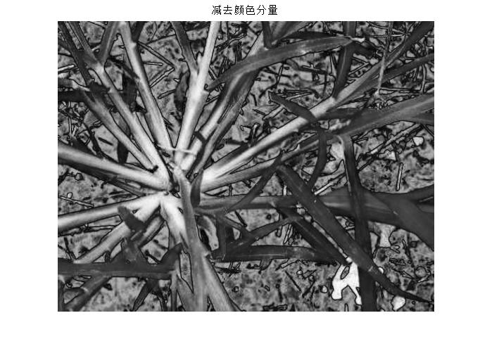
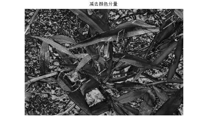
x1 = (r1+g1+b1)./3;
figure(1);
imshow(x1,[]);
title('Subtract color component');
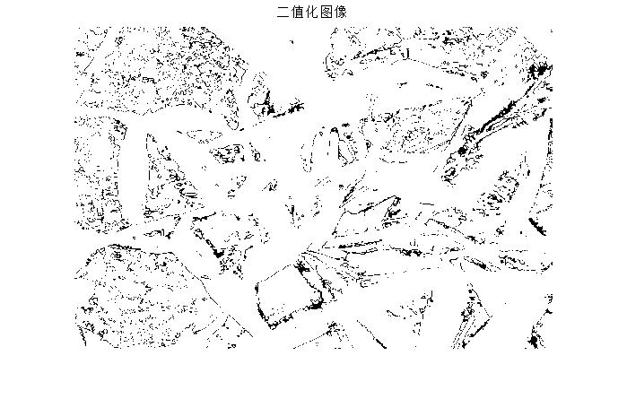
x1 = im2bw(x1,10/255);
figure(12);
imshow(x1,[]);
title('Binary image');
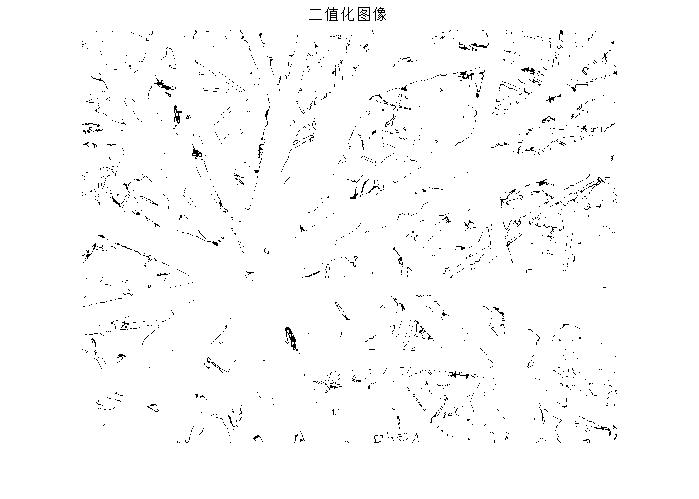
x1 = imopen(x1,se1);
x1 = imclose(x1,se2);
figure(2);
imshow(x1,[]);
title('After opening and closing operation');
y1 = adjvar(g1);
y1 = im2bw(y1,50/255);
figure(3);
imshow(y1,[]);
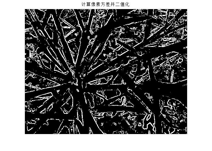
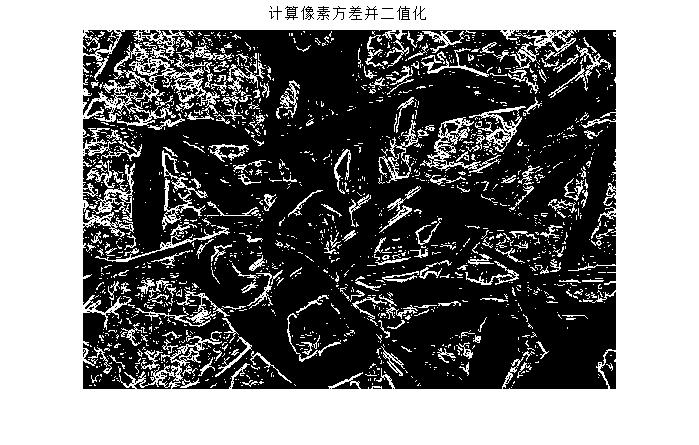
title('Calculate the pixel variance and binarize it');
x1 = -x1+1;
x1_labeled = bwlabel(x1);
%Show connected area
%Get the number of connected areas
x1_num = max(max(x1_labeled));
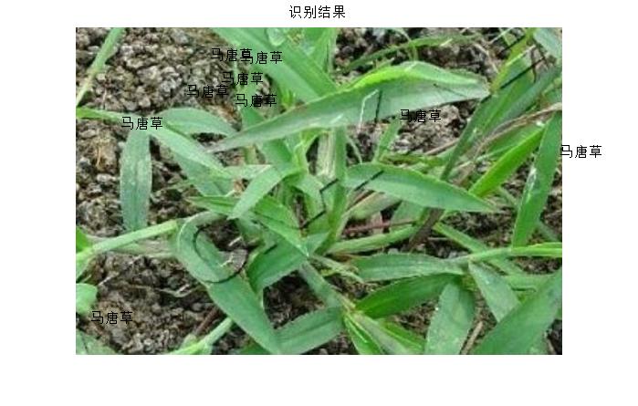
%Display the original image for later marking in the loop
figure(4);
imshow(I1);
title('Identification results');
for i = 1:x1_num
x1_idx = find(x1_labeled==i);
y1_idx = find(y1(x1_idx)==1);
%If the proportion of foreground pixels in the corresponding variance binary image in the current connected region to the total pixels in the connected region is greater than
%A certain threshold value is considered to be Tang grass, which is marked on the original image. The position to be marked is not accurately calculated here.
if(size(y1_idx,1)/size(x1_idx,1)>thresh1)
idx = x1_idx(floor(1+size(x1_idx,1)/2));
r = mod(idx,row1);
c = ceil(idx/row1);
text(c,r,'crabgrass ','color','black');
end
end
% --- Executes on button press in pushbutton4.
function pushbutton4_Callback(hObject, eventdata, handles)
% hObject handle to pushbutton4 (see GCBO)
% eventdata reserved - to be defined in a future version of MATLAB
% handles structure with handles and user data (see GUIDATA)
clear all
clc
close(gcf)
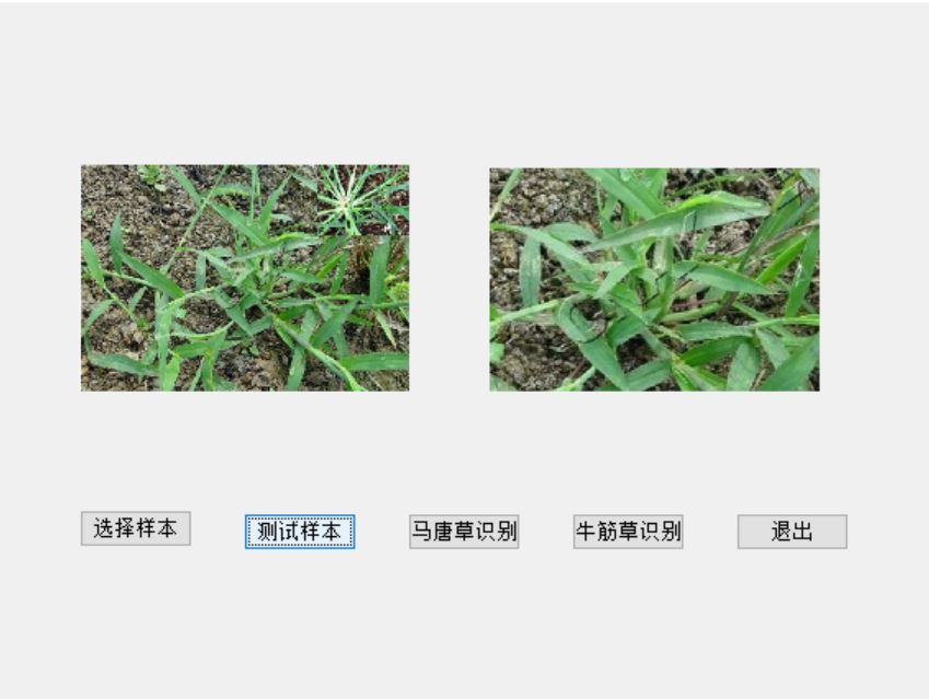
3, Operation results
4, Remarks
Version: 2014a