1. Theoretical basis

The propagation of light waves in free space can be described by a variety of theories. The most commonly used are Fresnel diffraction propagation, Fraunhofer diffraction propagation and angular spectrum theory.

In essence, the three are consistent, but the applicable conditions are different. Franchoffer diffraction is generally common in the far field or lens system in free space because of its harsh approximation conditions. The approximate condition of Fresnel diffraction is relatively simple and only needs to be in the paraxial region, which is generally applicable, but its calculation process is more complex than that of franchoffer. The propagation theory based on diffraction describes the light wave in the spatial domain, while the angular spectrum theory abstracts the light wave and analyzes it from the frequency domain. Any complex light wave can be considered as a plane light wave composed of various frequency components, and each plane light wave is a plane primitive. For example, complex light wavesCan be decomposed into

By observing the above formula, it can be found that the exponential term is actually a frequency ofandPlane light waves,Is its corresponding weight, which is traditionally called spectrum function. review Basic theory of Fourier transform , it can be found that the light wave function is obtained by inverse Fourier transform of the spectrum function, and the spectrum function is obtained by Fourier transform of the light wave. In MATLAB, the fast transformation can be realized by FFT (one-dimensional) or FFT 2 (two-dimensional).  

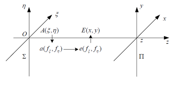Fig. 1 analysis process of angular spectrum theory

The general flow of analyzing problems by using angular spectrum theory is shown in Figure 1. Suppose there are two planes in free space, the input plane of z=0And the output plane of z=z, there is an arbitrary light wave function on the input surface, our purpose is to determine the light wave function when it is transmitted to the output surface in free space. First, yesThe spectrum is obtained by Fourier transform, multiply by the transfer functionThe spectrum of the output surface is obtainedThe wave function of the output surface is obtained by inverse Fourier transform. The key problem to be solved is to determine the transfer function.

Light wave functionThe frequency of isandThe composition of is, light wave functionThe corresponding component of is, comparing the two functions, we can find that the output side has one more term than the input side, and

So we can get the transfer function of free space

2. Example demonstration

According to the principle introduced above, some very interesting diffraction phenomena can be realized. It is assumed that a free-form surface is illuminated by a light source with normalized Gaussian amplitude distribution (size 10.24mm*10.24mm, wavelength 532nm, beam waist 5.32mm, as shown in Figure 2) (the maximum thickness is 3mm, and the surface shape is stored in z_g.mat matrix, as shown in Figure 3). Using the above analysis, we can get a Fresnel image after it propagates 200 mm in free space, as shown in Figure 4, which is very interesting.

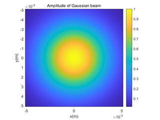Fig. 2 amplitude distribution of light source

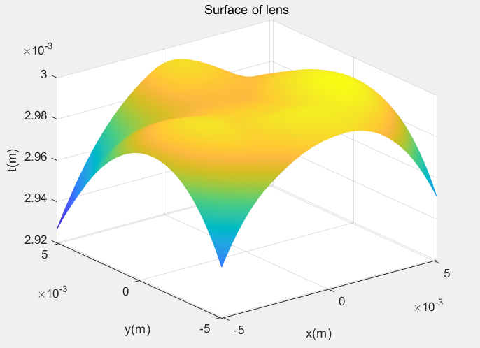Figure 3 free form surface

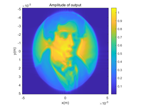Fig. 4 amplitude distribution of diffraction field

3.MATLAB code

clc;
clear all;
close all;
%% Generate the input Gaussian beam
mm=1e-3;
nm=1e-9;
lambda=532*nm;% wavelength
k=2*pi/lambda;% wavevector
n=1.494;% The rafractive index of freeform elements 
SL=10.24*mm ;% Side length
N=512*1;% samples for side length
dx=SL/N;%sample interval
d=200*mm;% The distance between the input and output planes
x = -0.5*SL:dx:0.5*SL-dx;% coordinate
y = x;
[X,Y]=meshgrid(x,y);
I_input=exp(-2*((X /(0.5* SL)).^2+(Y/(0.5* SL)).^2)); %The input Gaussian beam
figure;
imagesc(x,y,I_input);
axis square;
xlabel('x(m)');
ylabel('y(m)');
colorbar;
title('Amplitude of Gaussian beam');


%% phase modulataion by the freeform surface
load('z_g.mat');
OPD = 3*mm+(n-1)*z_g;
P_input  = exp(1i*k*OPD);
figure;mesh(X,Y,z_g);
title('Surface of lens');
xlabel('x(m)');
ylabel('y(m)');
zlabel('t(m)');
u1 = I_input.*P_input;

%% obtain the output field using Angular spectrum
fx=-1/(2*dx):1/SL:1/(2*dx)-1/SL;  %freq coords
[FX,FY]=meshgrid(fx,fx);
H=exp(1i*k*d*sqrt(1-(lambda*FX).^2-(lambda*FY).^2));  %trans func
H=fftshift(H);
U1=fft2(fftshift(u1));  %shift.fft source filed
U2=H.*U1;    %multiply
u2=fftshift(ifft2(U2));
figure;
imagesc(x,y,abs(u2));
axis square;
xlabel('x(m)');
ylabel('y(m)');
colorbar;
title('Amplitude of output');