1, Introduction

Moth flame optimization algorithm (MFO) is a new intelligent optimization algorithm proposed by Seyedali Mirjalili in 2015 [1]. The algorithm has the performance characteristics of strong parallel optimization ability, excellent global performance and not easy to fall into local extremum, which has gradually attracted the attention of academic and engineering circles.

1 algorithm principle
Moths use a special navigation mechanism of lateral positioning during night flight. In this mechanism, the moth flies by maintaining its fixed angle relative to the moon. Because the moon is very far away from the moth, the moth can fly in a straight line by using this approximate parallel light. Although this navigation mechanism is very effective for the moth, there are many artificial or natural point light sources in practice. Compared with the moon, this light source is very close to the moth. When the moth still flies at a fixed angle with the light source, it will lead to navigation failure and fatal spiral flight path.

In the MFO algorithm, it is assumed that the moth is the candidate solution to the problem, and the variable to be solved is the position of the moth in space. Therefore, by changing its own position vector, moths can fly in one-dimensional, two-dimensional, three-dimensional, or even higher dimensions. Since MFO algorithm is essentially a swarm intelligence optimization algorithm, moth population can be expressed in the matrix as follows:




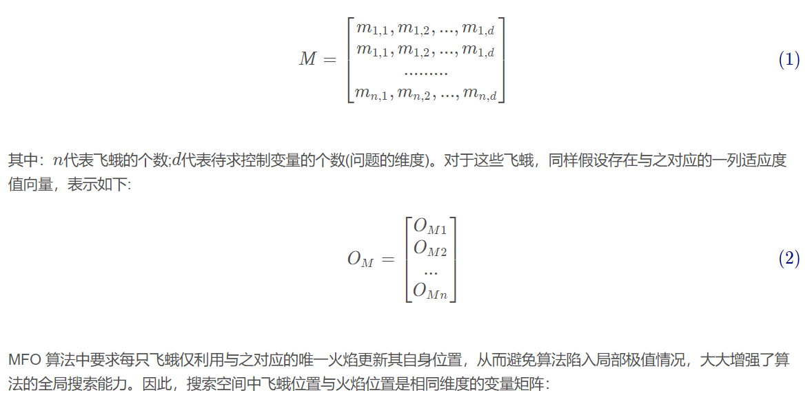
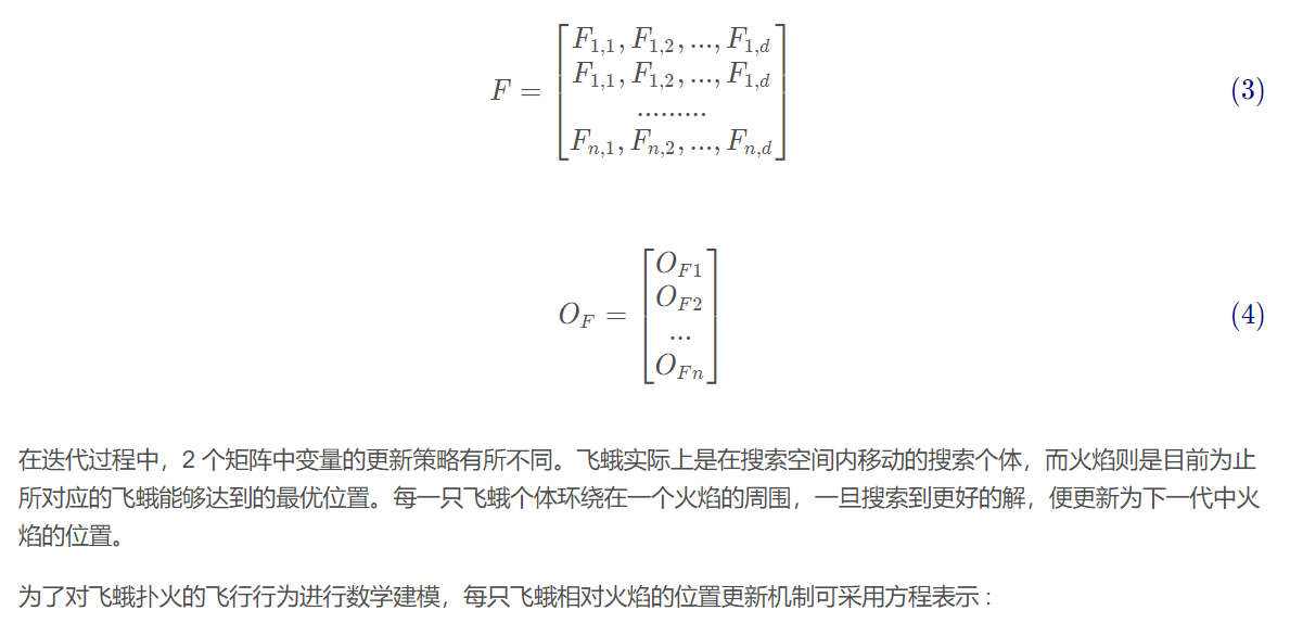
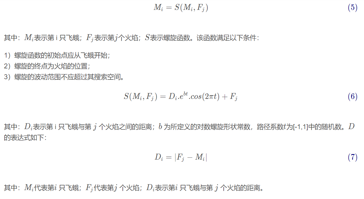
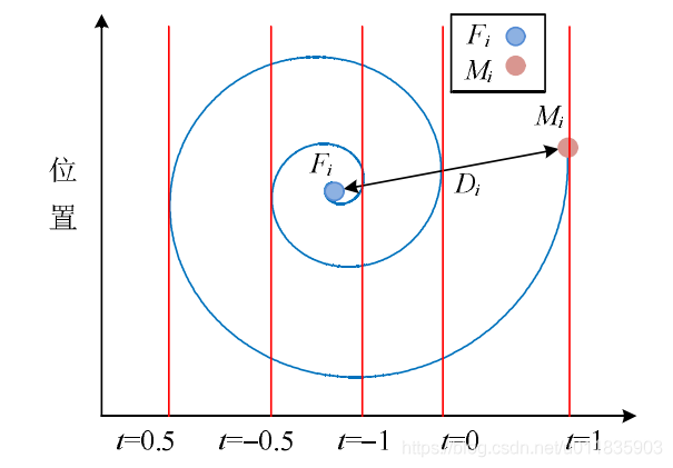
Figure 1 Logarithmic spiral and the space around the flame
Equation (6) simulates the spiral flight path of the moth. It can be seen that the next updated position of the moth is determined by the flame around it. As shown in Figure 1, the coefficient t tt in the spiral function represents the distance between the next position of the moth and the flame (t = − 1, t = - 1t = − 1 represents the position closest to the flame, and T = 1, t = 1t = 1 represents the farthest position). The spiral equation shows that moths can fly around the flame, not just in the space between them, so as to ensure the global search ability and local development ability of the algorithm. Figure 2 shows the position update model of moth around a flame. When a moth (blue horizontal line) flies around a flame (green horizontal line), if the fitness value of the updated moth position (black horizontal line) is better than the contemporary corresponding flame, its updated position will be selected as the position of the next generation flame (for example, as shown in label 2), so the moth has local development ability. The model has the following characteristics:

1) By modifying the parameter t tt, a moth can converge to any neighborhood of the flame.
2) The smaller the t tt, the closer the moth is to the flame.
3) As the moth gets closer to the flame, its renewal frequency around the flame becomes faster and faster.

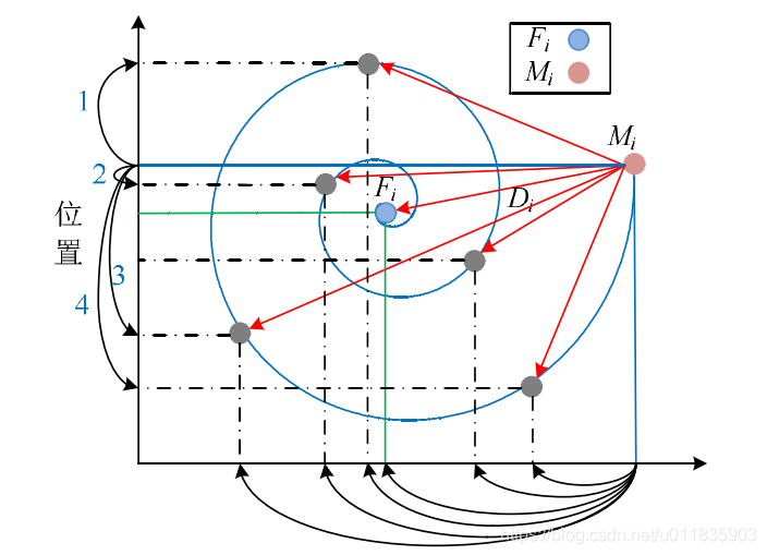
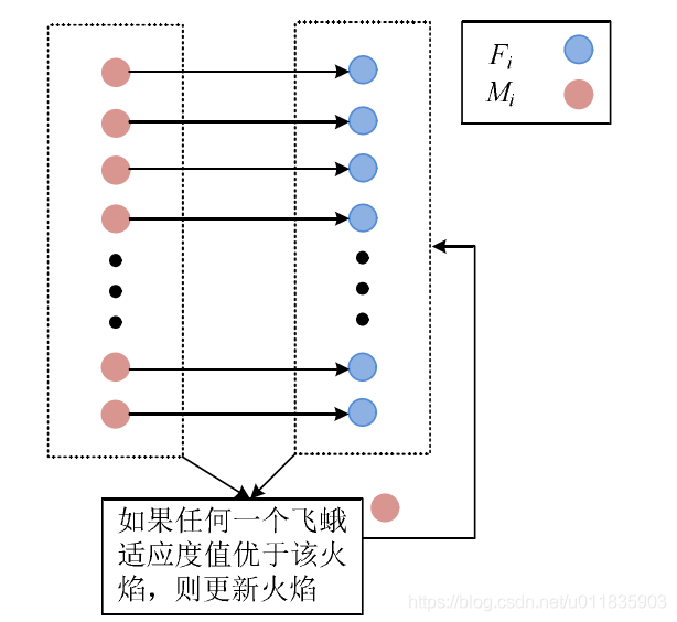
Figure 2 The possible position that a moth can reach by using logarithmic spiral according to the corresponding flame
The above flame position update mechanism can ensure the local development ability of moths around the flame. In order to improve the probability of finding a better solution, the currently found optimal solution is taken as the position of the next generation flame. Therefore, the flame position matrix F FF usually contains the currently found optimal solution. In the process of optimization, each moth updates its position according to the matrix F FF. The path coefficient t tt in MFO algorithm is a random number in [R, 1] [R, 1] [R, 1], and the variable r decreases linearly in [- 1, - 2] according to the number of iterations in the optimization iteration process. Through this treatment, with the iterative process, the moth will approach the flame in its corresponding sequence more accurately. After each iteration, the flame positions are reordered according to the fitness value to obtain the updated flame sequence, as shown in Figure 3. In the next generation, moths update their position according to the flame in their corresponding sequence.


2 algorithm flow
1) Initialization of MFO algorithm, setting parameters such as input optimal power flow control variable dimension d, moth population search scale n, maximum number of iterations T and logarithmic spiral shape constant b.
2) Initialize the variable to be solved, randomly generate the moth position in the search space, and evaluate the fitness value corresponding to each moth.
3) The spatial position of moths is sorted in the order of increasing fitness value and assigned to the flame as the spatial position of the flame in the first generation.
4) Use equation (5) to update the position of the current generation of moths.
5) Reorder the fitness values of the updated moth position and flame position, and select the spatial position with better fitness value to update the position of the next generation flame.
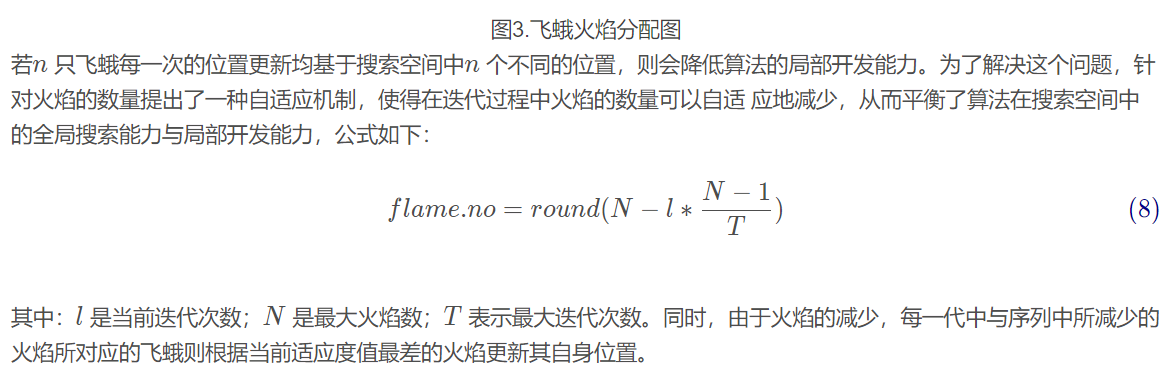
6) The number of flames is reduced by the adaptive mechanism of equation (8).
7) Return to step 6) and enter the next generation until the number of iterations meets the algorithm requirements.
10) Output and display the optimization results, and the program ends.

2, Source code

clear all
clc
SearchAgents_no=30;
Function_name='F1';
Max_iteration=1000;
[lb,ub,dim,fobj]=Get_Functions_details(Function_name);

[Best_score,Best_pos,cg_curve]=MFO(SearchAgents_no,Max_iteration,lb,ub,dim,fobj);
figure('Position',[284 214 660 290])
subplot(1,2,1);
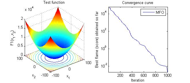
func_plot(Function_name);
title('Test function')
xlabel('x_1');
ylabel('x_2');
zlabel([Function_name,'(x_1,x_2)'])
function [lb,ub,dim,fobj] = Get_Functions_details(F)

switch F
    case 'F1'
        fobj=@F1;
        lb=-100;
        ub=100;
        dim=30;
    case 'F2'
    fobj=@F2;
    lb=-100;
    ub=100;
    dim=30;
    case 'F3'
    fobj=@F3;
    lb=-100;
    ub=100;
    dim=30;
    case 'F4'
    fobj=@F4;
    lb=-100;
    ub=100;
    dim=30;
    case 'F5'
    fobj=@F5;
    lb=-30;
    ub=30;
    dim=30;
    case 'F6'
    fobj=@F6;
    lb=-100;
    ub=100;
    dim=30;
    case 'F7'
    fobj=@F7;
    lb=-1.28;
    ub=1.28;
    dim=30;
    case 'F8'
    fobj=@F8;
    lb=-500;
    ub=500;
    dim=30;
    case 'F9'
    fobj=@F9;
    lb=-5.12;
    ub=5.12;
    dim=30;
    case 'F10'
    fobj=@F10;
    lb=-32;
    ub=32;
    dim=30;
    case 'F11'
    fobj=@F11;
    lb=-600;
    ub=600;
    dim=30;
    case 'F12'
    fobj=@F12;
    lb=-50;
    ub=50;
    dim=30;
    case 'F13'
    fobj=@F13;
    lb=-50;
    ub=50;
    dim=30;
    case 'F14'
    fobj=@F14;
    lb=-65.536;
    ub=65.536;
    dim=2;
    case 'F15'
    fobj=@F15;
    lb=-5;
    ub=5;
    dim=4;
    
    case 'F16'
    fobj=@F16;
    lb=-5;
    ub=5;
    dim=2;
    
    case 'F17'
    fobj=@F17;
    lb=[-5,0];
    ub=[10,15];
    dim=2;
    
    case 'F18'
    fobj=@F18;
    lb=-2;
    ub=2;
    dim=2;
    
    case 'F19'
    fobj=@F19;
    lb=0;
    ub=1;
    dim=3;
    
    case 'F20'
    fobj=@F20;
    lb=0;
    ub=1;
    dim=6;
    
    case 'F21'
    fobj=@F21;
    lb=0;
    ub=10;
    dim=4;
    
    case 'F22'
    fobj=@F22;
    lb=0;
    ub=10;
    dim=4;
    
    case 'F23'
    fobj=@F23;
    lb=0;
    ub=10;
    dim=4;
    
end
end
function o = F1(x)
o = sum(x.^2);
end
function o = F2(x)
    o=sum(abs(x))+prod(abs(x));
end

3, Operation results

4, Remarks

Version: 2014a