catalogue
2 two dimensional environment modeling
1 particle swarm optimization
yes Particle swarm optimization The summary is as follows: particle swarm optimization algorithm is a population-based search process, in which each individual (bird) is called a particle, which is defined as the feasible solution of the problem to be optimized in the D-dimensional search space, and has its historical optimal location and all particle The optimal position of memory, as well as speed. In each evolution generation, the particle information is combined to adjust the component of velocity on each dimension, and then used to calculate the new particle position. Particles constantly change their states in the multidimensional search space until they reach equilibrium or optimal state, or exceed the computational limit. Problem space The only connection between the different dimensions of is introduced through the objective function. Many empirical evidences have shown that the algorithm is a very effective optimization tool:

The principle formula of particle swarm optimization algorithm is not introduced here. Direct code:
function [ GBEST ,  cgCurve ] = PSO ( noP, maxIter,  problem, dataVis )

% Define the details of the objective function
nVar = problem.nVar;
ub = problem.ub;
lb = problem.lb;
fobj = problem.fobj;

% Extra variables for data visualization
average_objective = zeros(1, maxIter);
cgCurve = zeros(1, maxIter);
FirstP_D1 = zeros(1 , maxIter);
position_history = zeros(noP , maxIter , nVar );

% Define the PSO's paramters
wMax = 0.9;
wMin = 0.2;
c1 = 2;
c2 = 2;
vMax = (ub - lb) .* 0.2;
vMin  = -vMax;

% The PSO algorithm

% Initialize the particles
for k = 1 : noP
    Swarm.Particles(k).X = (ub-lb) .* rand(1,nVar) + lb;
    Swarm.Particles(k).V = zeros(1, nVar);
    Swarm.Particles(k).PBEST.X = zeros(1,nVar);
    Swarm.Particles(k).PBEST.O = inf;

    Swarm.GBEST.X = zeros(1,nVar);
    Swarm.GBEST.O = inf;
end


% Main loop
for t = 1 : maxIter

    % Calcualte the objective value
    for k = 1 : noP

        currentX = Swarm.Particles(k).X;
        position_history(k , t , : ) = currentX;


        Swarm.Particles(k).O = fobj(currentX);
        average_objective(t) =  average_objective(t)  + Swarm.Particles(k).O;

        % Update the PBEST
        if Swarm.Particles(k).O < Swarm.Particles(k).PBEST.O
            Swarm.Particles(k).PBEST.X = currentX;
            Swarm.Particles(k).PBEST.O = Swarm.Particles(k).O;
        end

        % Update the GBEST
        if Swarm.Particles(k).O < Swarm.GBEST.O
            Swarm.GBEST.X = currentX;
            Swarm.GBEST.O = Swarm.Particles(k).O;
        end
    end

    % Update the X and V vectors
    w = wMax - t .* ((wMax - wMin) / maxIter);

    FirstP_D1(t) = Swarm.Particles(1).X(1);

    for k = 1 : noP
        Swarm.Particles(k).V = w .* Swarm.Particles(k).V + c1 .* rand(1,nVar) .* (Swarm.Particles(k).PBEST.X - Swarm.Particles(k).X) ...
            + c2 .* rand(1,nVar) .* (Swarm.GBEST.X - Swarm.Particles(k).X);


        % Check velocities
        index1 = find(Swarm.Particles(k).V > vMax);
        index2 = find(Swarm.Particles(k).V < vMin);

        Swarm.Particles(k).V(index1) = vMax(index1);
        Swarm.Particles(k).V(index2) = vMin(index2);

        Swarm.Particles(k).X = Swarm.Particles(k).X + Swarm.Particles(k).V;

        % Check positions
        index1 = find(Swarm.Particles(k).X > ub);
        index2 = find(Swarm.Particles(k).X < lb);

        Swarm.Particles(k).X(index1) = ub(index1);
        Swarm.Particles(k).X(index2) = lb(index2);

    end

    if dataVis == 1
        outmsg = ['Iteration# ', num2str(t) , ' Swarm.GBEST.O = ' , num2str(Swarm.GBEST.O)];
        disp(outmsg);
    end

    cgCurve(t) = Swarm.GBEST.O;
    average_objective(t) = average_objective(t) / noP;

    fileName = ['Resluts after iteration # ' , num2str(t)];
    save( fileName)
end

GBEST = Swarm.GBEST;

if dataVis == 1
    iterations = 1: maxIter;

%% Draw the landscape
    figure

    x = -50 : 1 : 50;
    y = -50 : 1 : 50;

    [x_new , y_new] = meshgrid(x,y);

    for k1 = 1: size(x_new, 1)
        for k2 = 1 : size(x_new , 2)
            X = [ x_new(k1,k2) , y_new(k1, k2) ];
            z(k1,k2) = ObjectiveFunction( X );
        end
    end

    subplot(1,5,1)
    surfc(x_new , y_new , z);
    title('Search landscape')
    xlabel('x_1')
    ylabel('x_2')
    zlabel('Objective value')
    shading interp
    camproj perspective
    box on
    set(gca,'FontName','Times')


%% Visualize the cgcurve
    subplot(1,5,2);
    semilogy(iterations , cgCurve, 'r');
    title('Convergence curve')
    xlabel('Iteration#')
    ylabel('Weight')

%% Visualize the average objectives
    subplot(1,5,3)
    semilogy(iterations , average_objective , 'g')
    title('Average objecitves of all particles')
    xlabel('Iteration#')
    ylabel('Average objective')

 %% Visualize the fluctuations
    subplot(1,5,4)
    plot(iterations , FirstP_D1, 'k');
    title('First dimention in first Particle')
    xlabel('Iteration#')
    ylabel('Value of the first dimension')

 %% Visualize the search history
    subplot(1,5,5)
    hold on
    for p = 1 : noP
        for t = 1 : maxIter
            x = position_history(p, t , 1);
            y = position_history(p, t , 2);
            myColor = [0+t/maxIter  0 1-t/maxIter ];
            plot(x , y , '.' , 'color' , myColor );
        end
    end
    contour(x_new , y_new , z);
    plot(Swarm.GBEST.X(1) , Swarm.GBEST.X(2) , 'og');
    xlim([lb(1) , ub(1)])
    ylim([lb(2) , ub(2) ])
    title('search history')
    xlabel('x')
    ylabel('y')
    box on

    set(gcf , 'position' , [128         372        1634         259])


end
2 two dimensional environment modeling
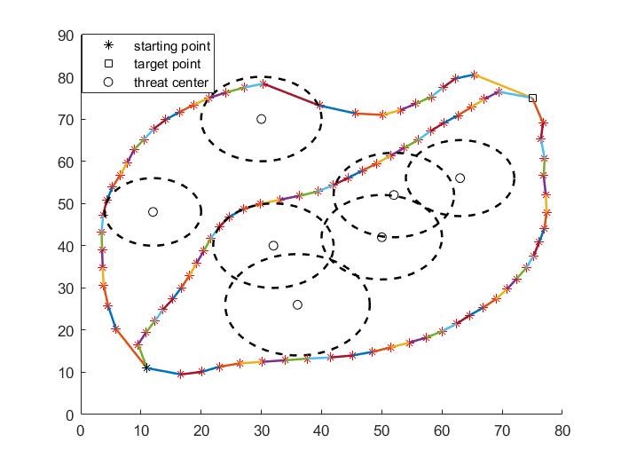
Two dimensional environment modeling can be regarded as the projection and simplification of the real three-dimensional environment. It is assumed that our moving objects work in a relatively horizontal environment and move at a uniform speed. The modeling diagram is as follows:
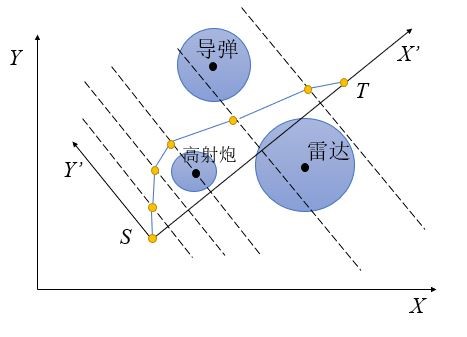
In the figure above, s and T are the starting point and end point respectively. The circle area is the area we need to avoid as much as possible in path planning (also known as threat). Its main parameters are threat center, threat radius and threat level (threat level is not shown in the schematic diagram). The line with yellow node as waypoint is a feasible planning path.
By designing a two-dimensional environment with different complexity, the effect of the algorithm in different harsh environments is tested. Here, three two-dimensional environments are used for the experiment:
%% case 1
radius = [10 10 8 12 9];
threat_lv = [2 10 1 2 3];
threat_center = [45,52;12,40;32,68;36,26;55,80];

%% case 2
radius = [10 10 8 12 9 10 10];
threat_lv = [2 10 1 2 5 2 4];
threat_center = [52,52;32,40;12,48;36,26;63,56;50,42;30,70];

%% case 3
radius = [10 18 10 12 10 11];
threat_lv = [5 5 5 5 5 5];
threat_center = [30,20;50,15;65,55;50,80;75,90;50,36];
3 path planning
Since the connecting line between the start point S and the end point T is not parallel to the X-axis, in order to facilitate calculation, we first rotate the coordinate axis, take the line where the segment ST is located as the new X-axis, and S as the origin of the new coordinate system.
Rotation matrix:
Design of path planning algorithm: we divide the new X-axis ST into D+1, which means that the path contains D yellow nodes. The X coordinates of D yellow nodes in the new coordinate system are known, and the Y coordinates need to be solved by Gray Wolf algorithm. Therefore, each feasible solution in the gray wolf algorithm is d-dimensional (that is, the Y coordinate containing D yellow nodes).
3.1 initialization
Particle swarm optimization algorithm needs to set several initial parameters, such as population number N (how many feasible solutions are randomly generated), iteration times, solution dimension D, and upper and lower bounds.
The population number N can be set according to the complexity of the actual problem or the size of the search space. Obviously, the larger N is not necessarily the better, because it will increase the time complexity of the algorithm.
The maximum number of iterations should not be too small and can be set through multiple experiments.
The upper and lower bounds (lb,ub) limit the range of solutions generated by the algorithm in the whole process. If we do not set the upper and lower bounds, the final generated path may be very outrageous. Although it does not pass through the threat area, the coverage may be very large and do not meet the actual requirements. In addition, the lower bound can limit the approximate area of the path.
3.2 fitness function
Here, we define the path cost as the accumulation of threat costs. The lower the belt price means the better the fitness. Only when the path passes through the threat area can we calculate the path cost of the section falling in the threat area:
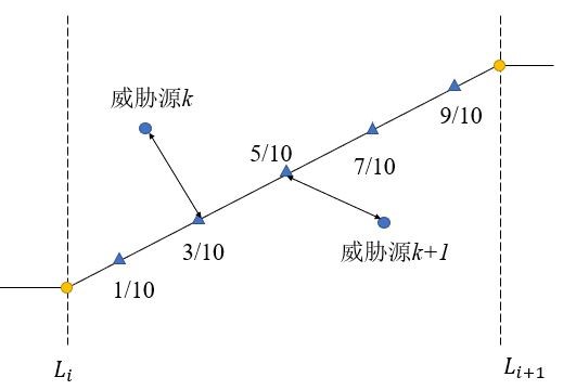
As shown in the figure above, the threat cost finally becomes the weighted sum of the threat costs of the five sampling points.
3.3 simulation results
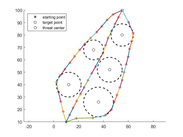
case1
case2
case3
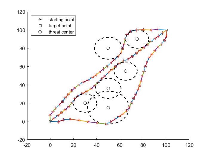
The three paths generated in the figure above are also required to have no conflict, and the paths cannot have intersection except the start point and end point. My solution is to assign different upper and lower bounds to the three paths to ensure that the regions will not coincide, and fundamentally ensure that the three paths will not intersect.
It can be seen that some paths in the simulation diagram pass through the threat area, which is caused by the randomness and upper and lower bounds of particle swarm optimization algorithm. Since the population initialization is generated randomly, and the initialization population will affect the final algorithm result, this randomness may make the algorithm fall into the local optimum, and the better the exploration mechanism of the algorithm, the stronger the ability to jump out of the local optimum, but it is inevitable. This is also the main disadvantage of the current swarm intelligence algorithm, but the global search is unrealistic, Searching the entire solution space is a waste of time.