1, Introduction
1 overview of genetic algorithm
Genetic Algorithm (GA) is a part of evolutionary computation. It is a computational model simulating Darwin's genetic selection and natural elimination of biological evolution process. It is a method to search the optimal solution by simulating the natural evolution process. The algorithm is simple, universal, robust and suitable for parallel processing.
2 characteristics and application of genetic algorithm
Genetic algorithm is a kind of robust search algorithm which can be used for complex system optimization. Compared with the traditional optimization algorithm, it has the following characteristics:
(1) Take the code of decision variable as the operation object. Traditional optimization algorithms often directly use the actual value of decision variables itself for optimization calculation, but genetic algorithm uses some form of coding of decision variables as the operation object. This coding method of decision variables enables us to learn from the concepts of chromosome and gene in biology in optimization calculation, imitate the genetic and evolutionary incentives of organisms in nature, and easily apply genetic operators.
(2) Directly take fitness as search information. The traditional optimization algorithm not only needs to use the value of the objective function, but also the search process is often constrained by the continuity of the objective function. It may also need to meet the requirement that "the derivative of the objective function must exist" to determine the search direction. The genetic algorithm only uses the fitness function value transformed from the objective function value to determine the further search range without other auxiliary information such as the derivative value of the objective function. Directly using the objective function value or individual fitness value can also focus the search range into the search space with higher fitness, so as to improve the search efficiency.
(3) Using the search information of multiple points has implicit parallelism. Traditional optimization algorithms often start from an initial point in the solution space. The search information provided by a single point is not much, so the search efficiency is not high, and it may fall into local optimal solution and stop; Genetic algorithm starts the search process of the optimal solution from the initial population composed of many individuals, rather than from a single individual. The, selection, crossover, mutation and other operations on the initial population produce a new generation of population, including a lot of population information. This information can avoid searching some unnecessary points, so as to avoid falling into local optimization and gradually approach the global optimal solution.
(4) Use probabilistic search instead of deterministic rules. Traditional optimization algorithms often use deterministic search methods. The transfer from one search point to another has a certain transfer direction and transfer relationship. This certainty may make the search less than the optimal store, which limits the application scope of the algorithm. Genetic algorithm is an adaptive search technology. Its selection, crossover, mutation and other operations are carried out in a probabilistic way, which increases the flexibility of the search process, and can converge to the optimal solution with a large probability. It has a good ability of global optimization. However, crossover probability, mutation probability and other parameters will also affect the search results and search efficiency of the algorithm, so how to select the parameters of genetic algorithm is an important problem in its application.
To sum up, because the overall search strategy and optimization search mode of genetic algorithm do not rely on gradient information or other auxiliary knowledge, and only need to solve the objective function and corresponding fitness function affecting the search direction, genetic algorithm provides a general framework for solving complex system problems. It does not depend on the specific field of the problem and has strong robustness to the types of problems, so it is widely used in various fields, including function optimization, combinatorial optimization, production scheduling problem and automatic control
, robotics, image processing (image restoration, image edge feature extraction...), artificial life, genetic programming, machine learning.
3 basic flow and implementation technology of genetic algorithm
Simple genetic algorithms (SGA) only uses three genetic operators: selection operator, crossover operator and mutation operator. The evolution process is simple and is the basis of other genetic algorithms.
3.1 basic flow of genetic algorithm
Generating a number of initial groups encoded by a certain length (the length is related to the accuracy of the problem to be solved) in a random manner;
Each individual is evaluated by fitness function. Individuals with high fitness value are selected to participate in genetic operation, and individuals with low fitness are eliminated;
A new generation of population is formed by the collection of individuals through genetic operation (replication, crossover and mutation) until the stopping criterion is met (evolutionary algebra gen > =?);
The best realized individual in the offspring is taken as the execution result of genetic algorithm.
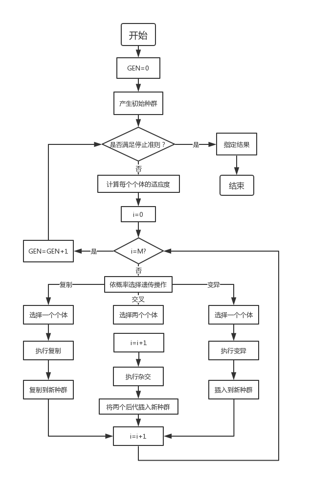
Where GEN is the current algebra; M is the population size, and i represents the population number.
3.2 implementation technology of genetic algorithm
Basic genetic algorithm (SGA) consists of coding, fitness function, genetic operators (selection, crossover, mutation) and operating parameters.
3.2.1 coding
(1) Binary coding
The length of binary coded string is related to the accuracy of the problem. It is necessary to ensure that every individual in the solution space can be encoded.
Advantages: simple operation of encoding and decoding, easy implementation of heredity and crossover
Disadvantages: large length
(2) Other coding methods
Gray code, floating point code, symbol code, multi parameter code, etc
3.2.2 fitness function
The fitness function should effectively reflect the gap between each chromosome and the chromosome of the optimal solution of the problem.
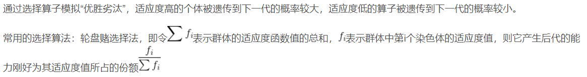
3.2.3 selection operator
3.2.4 crossover operator
Cross operation refers to the exchange of some genes between two paired chromosomes in some way, so as to form two new individuals; Crossover operation is an important feature of genetic algorithm, which is different from other evolutionary algorithms. It is the main method to generate new individuals. Before crossing, individuals in the group need to be paired. Generally, the principle of random pairing is adopted.
Common crossing methods:
Single point intersection
Two point crossing (multi-point crossing. The more crossing points, the greater the possibility of individual structure damage. Generally, multi-point crossing is not adopted)
Uniform crossing
Arithmetic Crossover
3.2.5 mutation operator
Mutation operation in genetic algorithm refers to replacing the gene values at some loci in the individual chromosome coding string with other alleles at this locus, so as to form a new individual.
In terms of the ability to generate new individuals in the operation process of genetic algorithm, crossover operation is the main method to generate new individuals, which determines the global search ability of genetic algorithm; Mutation operation is only an auxiliary method to generate new individuals, but it is also an essential operation step, which determines the local search ability of genetic algorithm. The combination of crossover operator and mutation operator completes the global search and local search of the search space, so that the genetic algorithm can complete the optimization process of the optimization problem with good search performance.
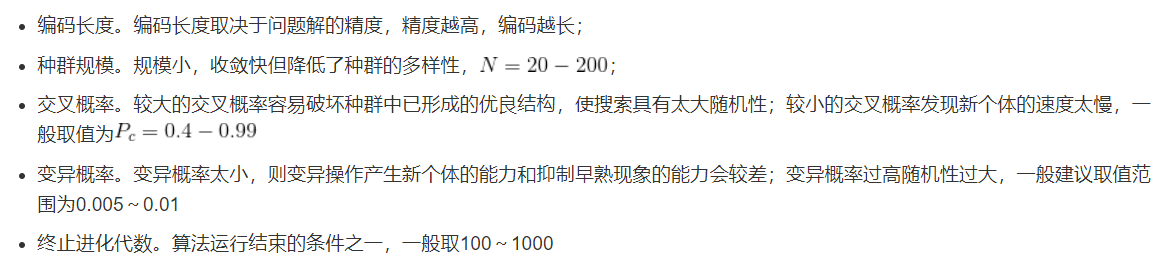
3.2.6 operating parameters
4 basic principle of genetic algorithm
4.1 mode theorem
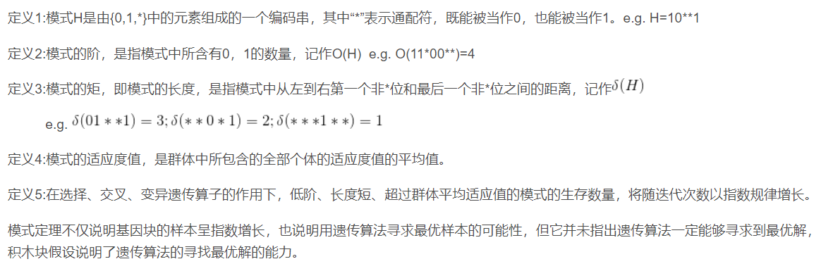
4.2 building block assumptions
Patterns with low order, short definition length and fitness value higher than the average fitness value of the population are called gene blocks or building blocks.
Building block hypothesis: individual gene blocks can be spliced together through genetic operators such as selection, crossover and mutation to form individual coding strings with higher fitness.
The building block hypothesis illustrates the basic idea of using genetic algorithm to solve various problems, that is, better solutions can be produced by directly splicing the building blocks together.
2, Source code
clear all;
clc;
format short g;
global D;
global q;
global q1;
global ss;
global E;
global L;
global ELL;
% test=xlsread('test.xlsx',1);
%
% position=test(:,2:3);

% data=[
%     100 100 0   0    0   40
%     60 100 10 0.2  0   3
%     20 110 15 0.3  0 4
%     160 150 21 0.3  1 6
%     160 110 16 0.4  0 4
%     30 20 25 0.3  1 4
%     100 60 22 0.2  0 6
%     100 170 15 0.1  0 5
%     30 10 12 0.4  0 6
%     60 50 15 0.3  1 7
%     160 160 20 0.2  0 6
%     50 140 23 0.3  0 6];
position=[18.70 15.29
       16.47 8.45
       20.07 10.14
       19.39 13.37
       25.27 14.24
       22.00 10.04
       25.47 17.02
       15.79 15.10
       16.60 12.38
       14.05 18.12
       17.53 17.38
       23.52 13.45
       19.41 18.13
       22.11 12.51
       11.25 11.04
       14.17 9.76
       24.00 19.89
       12.21 14.50];
% Distance matrix between distribution center and each demand point D
D=squareform(pdist(position(:,1:2),'euclidean'));
% Unit running cost of vehicle: h
% Fixed cost per vehicle: R.
% Vehicle speed v;
% Maximum loading capacity of the vehicle Qmax.
h=1;R=10;v=1;Qmax=200;epsilon=0.001;
R0=2;R1=0.8;
% Time matrix of vehicles traveling between the distribution center and each demand point T
T=D/v;

% Maximum number of iterations
Iter=30;
% Number of water droplets N
N=size(position,1);
% Speed update parameters:
av=1;bv=0.01;cv=1;
% Soil volume update parameters:
as=1;bs=0.01;cs=1;
% Local soil renewal weight coefficient
alpha=0.9;
% Global update weight coefficient
beta=0.9;
% Initial soil volume between any two points Initsoil
Initsoil=1000;
% Initial soil quantity matrix W ???
W=ones(N)*1000;
% Initial velocity of each droplet InitVel;
% InitVel=100;
InitVel=randperm(100,1);
% Global optimal objective function value
TotalZ=1000000;
% Global optimal path
TotalRoute=[];
% main program
t=0;
WaterDrop(1,N)=struct('SW',[],... % Initial soil mass matrix corresponding to water droplets
    'Source',[],... % The starting point of water droplets is 1; Distribution center
    'Target',[],... %
    'VisitNode',[],... % Accessed point sequence (Access path)
    'UnvisitNode',[],... % A collection of points that have not been accessed
    'Vel',[],... % Initial velocity of water droplets
    'Soil',[],... % Initial amount of soil carried by water droplets
    'Q',[],... % Loading of water droplets at departure
    'S',[],... % Water drop arrival source(k)The hour of the hour
    'ZZ',[],... %Initial value of objective function corresponding to water drop
    'FK',[]); % from source(k)The collection of the next demand points that can go FV
%  q=test(:,4); % Demand at each demand point
% q1=TestData(:,5);
q=[0 6 5 11 6 3 8 5 6 4 5 7 6 10 9 4 7 8 ]';
% q1=[0 3.6 2	4.6	3.6	2.4	4.8	3 3.6 2.4 3	4.2	3.6	4 5.4 2.6 2.4 3]';
%  ss=test(:,7); % Service time per demand point
ss=[0  1.8  1.0  2.3  1.8  1.2  2.4  1.5  1.8  1.2  1.5  2.1  1.8  2.0  2.7  1.3  1.2  1.5]';
E=[0  5.0  4  1  2.0  5  2  1 3  1  2  2.0  2  3  2  3  2  1]';
L=[40  20  15  20  20  15  18  24  27  20  16  20  10  25  28  24.0  20  23]';
%
% E=test(:,5); % Lower limit of time window for each demand point
%  L=test(:,6); % Upper limit of time window at each demand point
ELL=L-E;
% EP=test(:,8);
% LP=test(:,9);
I=1:N;
while t < Iter
     clc
    fprintf('The first%d Secondary evolution\n',t+1) ;
    % Set the initial dynamic variable:
    % Optimal objective function value of this iteration
    Z=1000000;
    % The optimal path of this iteration
    Route=[];
    for k=1:N
        WaterDrop(k).SW=W;
        WaterDrop(k).Source=1;
        WaterDrop(k).VisitNode=[1];
        WaterDrop(k).UnvisitNode=I;
        WaterDrop(k).Vel= InitVel;
        % Initial amount of soil carried by water droplets
        WaterDrop(k).Soil=0;
        % Loading of water droplets at departure
        WaterDrop(k).Q(WaterDrop(k).Source)=0;
        % Water drop arrival source(k)The time of the hour;
        WaterDrop(k).S(WaterDrop(k).Source)=0;
        % The first k Initial value of objective function corresponding to water droplets
        WaterDrop(k).ZZ=0;
    end
    for k=1:N
        while WaterDrop(k).Source~=1 || ~isequal(WaterDrop(k).UnvisitNode,[1])
            WaterDrop(k).FK=[];
            if WaterDrop(k).Source==1
                alt=2;
            else
                alt=1;
            end
            for i=alt:length(WaterDrop(k).UnvisitNode)

                   WaterDrop(k).Q(WaterDrop(k).UnvisitNode(i))=WaterDrop(k).Q(WaterDrop(k).Source)+q(WaterDrop(k).UnvisitNode(i));
                   % judge i Is the load capacity of the point less than the maximum load of the vehicle and reached i Is the time of the hour i Point within the required time window
                    if WaterDrop(k).Q(WaterDrop(k).UnvisitNode(i))<Qmax;
                        WaterDrop(k).FK=[WaterDrop(k).FK,WaterDrop(k).UnvisitNode(i)];
                    end
            end
%             for i=alt:N
%                 if ismember(i,WaterDrop(k).UnvisitNode)
%                % if sum(ismember(WaterDrop(k).UnvisitNode,i))
%                     WaterDrop(k).Q(i)=WaterDrop(k).Q(WaterDrop(k).Source)+q(i);
%                     WaterDrop(k).S(i)=WaterDrop(k).S(WaterDrop(k).Source)+ss(WaterDrop(k).Source)+T(WaterDrop(k).Source,i);
%                    % judge i Is the load capacity of the point less than the maximum load of the vehicle and reached i Is the time of the hour i Point within the required time window
%                     if WaterDrop(k).Q(i)<Qmax && WaterDrop(k).S(i)>=E(i) && WaterDrop(k).S(i)<=L(i)
%                         WaterDrop(k).FK=[WaterDrop(k).FK,i];
%                     end
%                 end
%             end
            if isempty(WaterDrop(k).FK)
                WaterDrop(k).Target=1;
            else
                % Calculate the probability of going to the next demand point that can be served
                % Judge from source(k)Is the minimum value of soil quantity on the path to the next demand point that can be served less than 0
                Minsoil=0;
                for u=1:length(WaterDrop(k).FK)
                    if WaterDrop(k).SW(WaterDrop(k).Source,WaterDrop(k).FK(u))<Minsoil
                        Minsoil=WaterDrop(k).SW(WaterDrop(k).Source,WaterDrop(k).FK(u));
                    end
                end
                % Find the function corresponding to the next service demand point f Sum of (you can add improvements and adjust node selection probability)
                SumF=0;
                for u=1:length(WaterDrop(k).FK)
                    g(WaterDrop(k).Source,WaterDrop(k).FK(u))=WaterDrop(k).SW(WaterDrop(k).Source,WaterDrop(k).FK(u))-Minsoil;
                    f(WaterDrop(k).Source,WaterDrop(k).FK(u))=1/(0.01+g(WaterDrop(k).Source,WaterDrop(k).FK(u)));
                    SumF=SumF+f(WaterDrop(k).Source,WaterDrop(k).FK(u));
                end

                 % Calculate the probability corresponding to the service demand point
                 P=[];
                 U=[];
                 for u=1:length(WaterDrop(k).FK)
                     P=[P,f(WaterDrop(k).Source,WaterDrop(k).FK(u))/SumF];
                     U=[U,WaterDrop(k).FK(u)];
                 end
                 % According to probability P(source(k),u), By Roulette FV(k) Randomly select a point in the set
                WaterDrop(k).Target=U(RoutedGame(P));
            end
            % Update the speed of water droplets
            WaterDrop(k).Vel=WaterDrop(k).Vel+av/(bv+cv*WaterDrop(k).SW(WaterDrop(k).Source,WaterDrop(k).Target)^2);
            Maxtime=max(epsilon,WaterDrop(k).Vel);
            % Calculate the time required for water droplets to flow to the target point
            TT(WaterDrop(k).Source,WaterDrop(k).Target)=D(WaterDrop(k).Source,WaterDrop(k).Target)/Maxtime;
            % Calculate the increment of soil carried by water droplets
            DeltaSW(WaterDrop(k).Source,WaterDrop(k).Target)= as/(bs+cs*TT(WaterDrop(k).Source,WaterDrop(k).Target)^2);
            % Update the amount of soil on the path through which water droplets flow
            WaterDrop(k).SW(WaterDrop(k).Source,WaterDrop(k).Target)=...
                (1-alpha)*WaterDrop(k).SW(WaterDrop(k).Source,WaterDrop(k).Target)-alpha*DeltaSW(WaterDrop(k).Source,WaterDrop(k).Target);
            % Update the amount of soil carried by water droplets
            WaterDrop(k).Soil=WaterDrop(k).Soil+DeltaSW(WaterDrop(k).Source,WaterDrop(k).Target);
%             %Penalty coefficient for early arrival and late arrival
%             cfe1=0;
%             cfe2=0;
%             cfe0=0;
            WaterDrop(k).S(WaterDrop(k).Target)=WaterDrop(k).S(WaterDrop(k).Source)+ss(WaterDrop(k).Source)+T(WaterDrop(k).Source,WaterDrop(k).Target);
%             if WaterDrop(k).S(WaterDrop(k).Target)<E
%                 cfe1=EP(WaterDrop(k).Target)*abs(E-WaterDrop(k).Target);
%             elseif WaterDrop(k).S(WaterDrop(k).Target)>L
%                 cfe1=LP(WaterDrop(k).Target)*abs(WaterDrop(k).Target-L);
%             end
%             cfe0=cfe1+cfe2;
            if  WaterDrop(k).Target==1
                % (Orderly Collection) delivery vehicles return to the distribution center
                WaterDrop(k).VisitNode=[WaterDrop(k).VisitNode,WaterDrop(k).Target];
                % Increase the fixed cost of using one vehicle in the objective function (indicating that a loop of one vehicle is formed)
                WaterDrop(k).ZZ=WaterDrop(k).ZZ+h*D(WaterDrop(k).Source,WaterDrop(k).Target)+D(WaterDrop(k).Source,WaterDrop(k).Target)*(R0+R1*(q(WaterDrop(k).Target)))+R;
                WaterDrop(k).Source=WaterDrop(k).Target;
                WaterDrop(k).Q(WaterDrop(k).Source)=0;
                WaterDrop(k).S(WaterDrop(k).Source)=0;
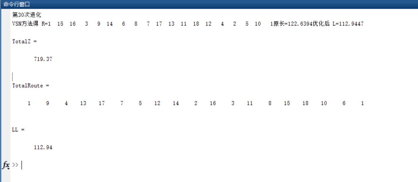
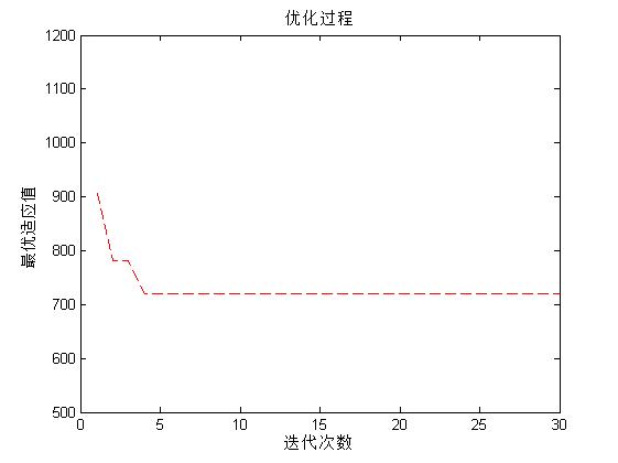
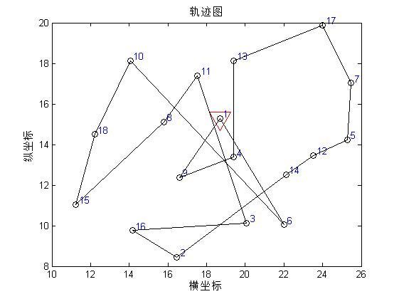
3, Operation results
4, Remarks
Version: 2014a