1 genetic algorithm
Step 1: the setting of relevant parameters generally includes coding length L, population size M, number of iterations G, crossover rate Pc, mutation rate Pm, etc.
Step 2: the solution in the mathematical model cannot be directly used in the algorithm. The solution needs to be processed to construct the chromosome of the fitness function.
Step 3: M individuals are randomly generated to form the initial population Po, and the individuals are orderly distributed in the solution space. Each individual is a solution corresponding to the problem.
Step 4: calculate the fitness of each individual, and carry out selection and other operations in the population according to the fitness.
Step 5: according to the fitness of each individual, select individuals with high fitness for individual selection and other operations. The commonly used methods include roulette and so on.
Step 6: set the crossover rate Pc to control the crossover operation of the parent chromosome, and the crossed individual will enter the new species group instead of the parent.
Step 7: set the mutation rate Pm and control the mutation operation of the parent chromosome. Mutations can lead to the reappearance of genes that do not appear in the population or are eliminated in the selection process, and mutant individuals replace their parents into the new population.
Step 8: judge whether the updated population after the selection, crossover and mutation operations of the next iteration meets the termination conditions. If not, go back to step 4 for cyclic iteration; If it is satisfied, the algorithm will be stopped, and the maximum number of iterations is usually used as the termination criterion.
Step 9: decode the chromosome that meets the termination conditions to obtain the optimal solution of the problem. According to the above steps, we can know the basic process of genetic algorithm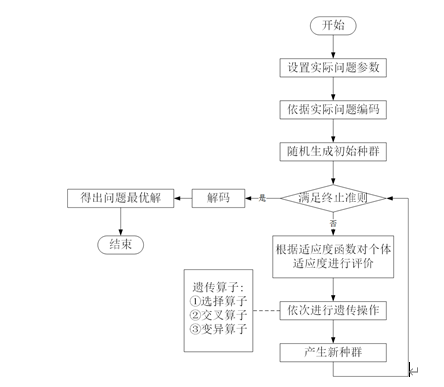
2 code display
%Genetic algorithm solution TSP problem(The program is redesigned for the selection operation)
%Input:
%D Distance matrix
%NIND Is the number of populations
%X The parameter is the coordinates of 34 cities in China(Initial setting)
%MAXGEN To stop algebra, inherit to the second MAXGEN Time substitution program stop,MAXGEN The specific value of depends on the scale of the problem and the time spent
%m Acceleration index for value elimination,It is better to take 1,2,3,4,Not too big
%Pc Crossover probability
%Pm Variation probability
%Output:
%R Is the shortest path
%Rlength Is the path length
clear
clc
close all
%% Load data %%Genetic parameters
load zby;%City coordinate location
NIND=50; %Population size
MAXGEN=200;
Pc=0.9; %Crossover probability
Pm=0.2; %Variation probability
GGAP=0.9; %generation gap(Generation gap)
load('D.mat')
D=D; %Generate distance matrix
N=size(D,1);
%% Initialize population
Chrom=InitPop(NIND,N,D);
%% Draw all coordinate points on the two-dimensional diagram
% figure
% plot(X(:,1),X(:,2),'o');
% pause(2)
% %% Draw the road map of random solution
% DrawPath(Chrom(1,:),X)
%
%% Route and total distance of output random solution
% disp('A random value in the initial population:')
% OutputPath(Chrom(1,:));
% Rlength=PathLength(D,Chrom(1,:));
% disp(['Total distance:',num2str(Rlength)]);
% disp('~~~~~~~~~~~~~~~~~~~~~~~~~~~~~~~~~~~~~~~~~~~~~~~~~~~~~~~~~~~~~~~~')
pause(1)
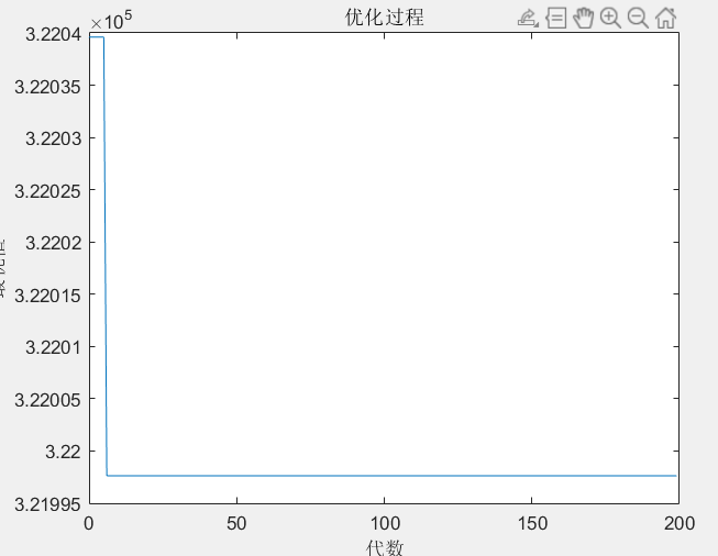
%% optimization
gen=0;
figure;
hold on;box on
xlim([0,MAXGEN])
title('Optimization process')
xlabel('Algebra')
ylabel('optimal value')
ObjV=PathLength(D,Chrom); %Calculate route length
preObjV=min(ObjV);
while gen<MAXGEN
%% Calculate fitness
ObjV=PathLength(D,Chrom); %Calculate route length
% fprintf('%d %1.10f\n',gen,min(ObjV))
line([gen-1,gen],[preObjV,min(ObjV)]);pause(0.0001)
preObjV=min(ObjV);
FitnV=Fitness(ObjV);
%% choice
SelCh=Select(Chrom,FitnV,GGAP);
%% Cross operation
% SelCh=cross(SelCh,FitnV,D);
SelCh=Recombin(SelCh,Pc);
%% variation
SelCh=Multate(SelCh,Pm);
%% New populations of reinsertion Progenies
Chrom=Reins(Chrom,SelCh,ObjV);
for j=1:NIND
cdd=Chrom(j,:);
if cdd(1,1)~=1
cc=find(cdd==1);
cdd(cc)=[];
Chrom(j,:)=[1,cdd];
end
end
%% Update iterations
gen=gen+1 ;
end
%% Draw the road map of the optimal solution
ObjV=PathLength(D,Chrom); %Calculate route length
[minObjV,minInd]=min(ObjV);
minchr=Chrom(minInd(1),:);
acs=find(minchr==11);
minch=minchr(1:acs);
DrawPath(minch,X)
%% Route and total distance of output optimal solution
disp('Optimal solution:')
p=OutputPath(minch);
disp(['Total distance:',num2str(ObjV(minInd(1)))]);
disp('-------------------------------------------------------------')
[~,cc]=size(minch);
disp(['Charging times:',num2str(cc-2)]);
disp('-------------------------------------------------------------')
disp(['Remaining power:',num2str(100-D(minch(end-1),minch(end))),'%']);
disp('-------------------------------------------------------------')
disp(['Time:',num2str(ObjV(minInd(1))/70+1*(D(minch(1),minch(2)))/100)]);
Optimization results
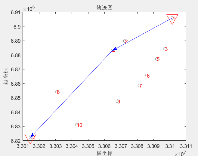

ans =
10 4 2 3 1 5 8 11 9 7 6
Optimal solution:
1—>4—>11
Total distance: 321997.6348
Code download https://www.cnblogs.com/matlabxiao/p/14883637.html