principle
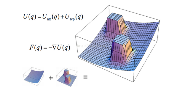
Establish the potential field manually, set the obstacle as repulsion and the target as attraction, add the force vectors, and finally calculate the direction of the resultant force.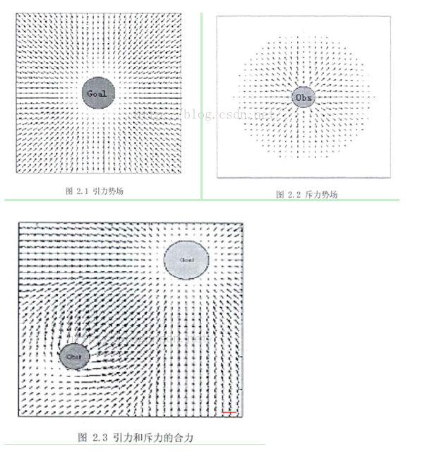
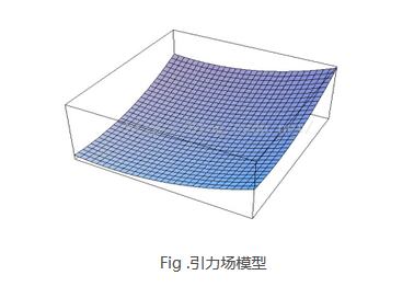
gravitational field
Common gravitational functions: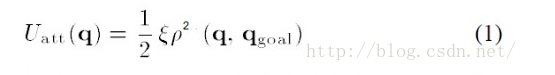
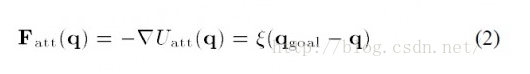
there ε Is a scale factor ρ (q,q_goal) indicates the distance between the current state of the object and the target. If there is a gravitational field, then gravity is the derivative of the gravitational field to the distance (analogy physics W=FX):
Repulsive field
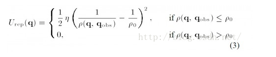
Formula (3) is a traditional repulsion field formula. In the formula η Is the repulsion scale factor, ρ (q,q_obs) represents the distance between the object and the obstacle. ρ_ 0 represents the influence radius of each obstacle. In other words, at a certain distance, the obstacle has no repulsive effect on the object.
Repulsion is the gradient of the repulsive field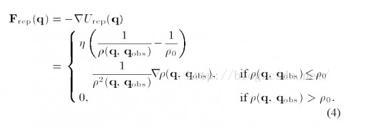
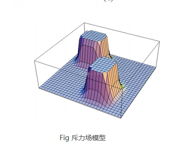
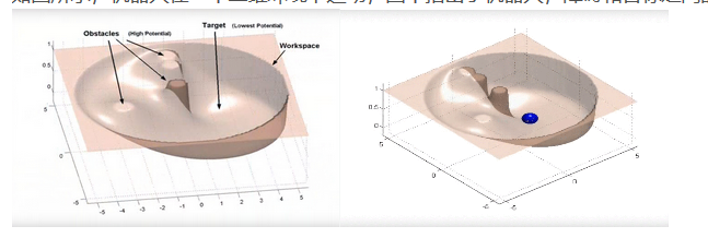
The total field is the superposition of the gravitational field in the case of repulsion, that is, U=U_att+U_rep, the total force is also the superposition of the corresponding component force, as shown in the following figure:
advantage:
Simple and practical, with good real-time performance
The structure is simple and convenient for the real-time control of the bottom layer. It has been widely used in real-time barrier and smooth trajectory control
Disadvantages:
- When the target point is far away, the gravity will become particularly large. Under relatively small repulsion, the object path may encounter obstacles
- When there is an obstacle near the target point, the repulsion force will be very large and the gravity is relatively small, so it is difficult for the object to reach the target point
- At a certain point, the gravitational repulsion is just equal and the direction is opposite. The object is easy to fall into local optimal solution or oscillation
- Easy to fall into local optimal solution
improvement:
- The problem of encountering obstacles can be solved by modifying the gravity function to avoid excessive gravity caused by too large distance.
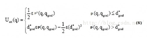 Compared with formula (1), formula (5) increases the scope limit. d*_goal gives a threshold that defines the distance between the target and the object. The corresponding gradient, that is, gravity, becomes:
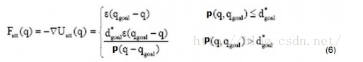
- A new repulsion function is introduced to solve the problem of unreachable target caused by obstacles near the target point
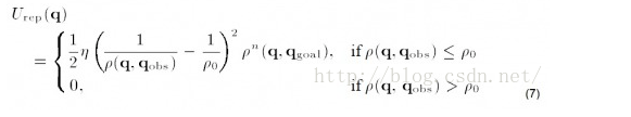
Here, on the basis of the original repulsion field, the influence of the distance between the target and the object is added (n is a positive number, I see n=2 in a literature). Intuitively, when the object approaches the target, although the repulsion field increases, the distance decreases, so it can drag the repulsion field to a certain extent
The corresponding repulsion becomes: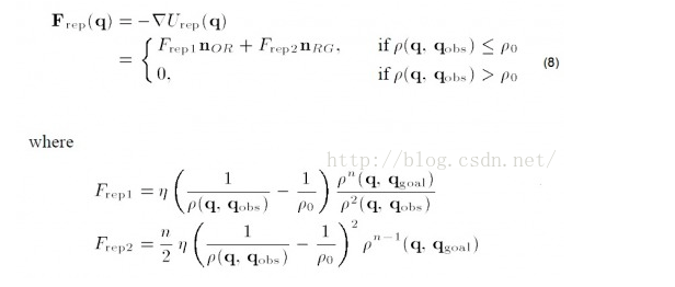
Therefore, we can see that gravity here is divided into two parts. We should pay special attention to it when programming
- The local optimal problem is a big problem of the artificial potential field method. Here, the object can jump out of the local optimal value by adding a random disturbance. The solution is similar to the local optimal value of the gradient descent method.
function varargout = AFM(varargin)
% AFM MATLAB code for AFM.fig
% AFM, by itself, creates a new AFM or raises the existing
% singleton*.
%
% H = AFM returns the handle to a new AFM or the handle to
% the existing singleton*.
%
% AFM('CALLBACK',hObject,eventData,handles,...) calls the local
% function named CALLBACK in AFM.M with the given input arguments.
%
% AFM('Property','Value',...) creates a new AFM or raises the
% existing singleton*. Starting from the left, property value pairs are
% applied to the GUI before AFM_OpeningFcn gets called. An
% unrecognized property name or invalid value makes property application
% stop. All inputs are passed to AFM_OpeningFcn via varargin.
%
% *See GUI Options on GUIDE's Tools out. Choose "GUI allows only one
% instance to run (singleton)".
%
% See also: GUIDE, GUIDATA, GUIHANDLES
% Edit the above text to modify the response to help AFM
% Last Modified by GUIDE v2.5 28-Nov-2013 20:49:25
% Begin initialization code - DO NOT EDIT
gui_Singleton = 1;
gui_State = struct('gui_Name', mfilename, ...
'gui_Singleton', gui_Singleton, ...
'gui_OpeningFcn', @AFM_OpeningFcn, ...
'gui_OutputFcn', @AFM_OutputFcn, ...
'gui_LayoutFcn', [] , ...
'gui_Callback', []);
if nargin && ischar(varargin{1})
gui_State.gui_Callback = str2func(varargin{1});
end
if nargout
[varargout{1:nargout}] = gui_mainfcn(gui_State, varargin{:});
else
gui_mainfcn(gui_State, varargin{:});
end
% End initialization code - DO NOT EDIT
% --- Executes just before AFM is made visible.
function AFM_OpeningFcn(hObject, eventdata, handles, varargin)
% This function has no output args, see OutputFcn.
% hObject handle to figure
% eventdata reserved - to be defined in a future version of MATLAB
% handles structure with handles and user data (see GUIDATA)
% varargin command line arguments to AFM (see VARARGIN)
% Choose default command line output for AFM
handles.output = hObject;
% Update handles structure
guidata(hObject, handles);
% UIWAIT makes AFM wait for user response (see UIRESUME)
% uiwait(handles.figure1);
% --- Outputs from this function are returned to the command line.
function varargout = AFM_OutputFcn(hObject, eventdata, handles)
% varargout cell array for returning output args (see VARARGOUT);
% hObject handle to figure
% eventdata reserved - to be defined in a future version of MATLAB
% handles structure with handles and user data (see GUIDATA)
% Get default command line output from handles structure
varargout{1} = handles.output;
% --- Executes during object creation, after setting all properties.
function axes4_CreateFcn(hObject, eventdata, handles)
Xo=[0 0];%Starting point position
k=1;%Gain coefficient required to calculate gravity
m=1;%Calculate the gain coefficient of repulsion
%n=3;%Number of obstacles
longth=1.2;%step
J=2000;%Number of loop iterations
%If the expected goal cannot be achieved, it may also be related to the initial gain coefficient, Po Improper setting.
K=0;%initialization
%[m_Obs,m_ObsR]=Obs_Generate([5 10],[20 80],[10 80],n);
Xj=Xo;%j=1 At the beginning of the cycle, assign the starting coordinates of the vehicle to Xj
axis([-20 120 -20 120]);
axis equal;
hold on;
axis off;
%set(gcf,'color','y')
%fill([-10,110,110,-10],[-10 -10 110 110],'w')
fill([-20,120,120,-20],[-20 -20 120 120],'y')
%title ('Artificial potential field path planning');
text(-5,-5,' Start','FontSize',12);
fill([95,120,120,95],[-20 -20 10 10],'w')
text(100,5,'Notes:','FontSize',12)
plot(101,-5,'sb','markerfacecolor','b');
text(101,-5,' Robot','FontSize',12);
plot(101,-15,'om','markerfacecolor','m');
text(101,-15,' Ball','FontSize',12);
plot(0,0,'bs')
car=plot(0,0,'sb','markerfacecolor','b');
%car_name=text(0,0,' ','FontSize',12);
object=plot(0,100,'om','markerfacecolor','m');
%object_name=text(0,100,' Ball','FontSize',12);
but=1;
x_obs=1;
y_obs=1;
% hObject handle to axes4 (see GCBO)
% eventdata reserved - to be defined in a future version of MATLAB
% handles empty - handles not created until after all CreateFcns called
% Hint: place code in OpeningFcn to populate axes4
% --- Executes on button press in pushbutton1.
function pushbutton1_Callback(hObject, eventdata, handles)
%main
%%%%%%%%%%%%%%%%%%%%%Initialization parameters%%%%%%%%%%%%%%%%%%%%%%%%%%%%%%%5
Xo=[0 0];%Starting point position
k=1;%Gain coefficient required to calculate gravity
m=1;%Calculate the gain coefficient of repulsion
%n=3;%Number of obstacles
longth=1.2;%step
%Number of loop iterations
J=2000;
%If the expected goal cannot be achieved, it may also be related to the initial gain coefficient, Po Improper setting.
K=0;%initialization
%[m_Obs,m_ObsR]=Obs_Generate([5 10],[20 80],[10 80],n);
Xj=Xo;%j=1 At the beginning of the cycle, assign the starting coordinates of the vehicle to Xj
axis([-20 120 -20 120]);
axis equal;
hold on;
axis off;
%set(gcf,'color','y')
%fill([-10,110,110,-10],[-10 -10 110 110],'w')
fill([-20,120,120,-20],[-20 -20 120 120],'y')
%title ('Artificial potential field path planning');
text(-5,-5,' Start','FontSize',12);
fill([95,120,120,95],[-20 -20 10 10],'w')
text(100,5,'Notes:','FontSize',12)
plot(101,-5,'sb','markerfacecolor','b');
text(101,-5,' Robot','FontSize',12);
plot(101,-15,'om','markerfacecolor','m');
text(101,-15,' Ball','FontSize',12);
plot(0,0,'bs')
car=plot(0,0,'sb','markerfacecolor','b');
%car_name=text(0,0,' ','FontSize',12);
object=plot(0,100,'om','markerfacecolor','m');
%object_name=text(0,100,' Ball','FontSize',12);
but=1;
x_obs=1;
y_obs=1;
%pause(1);
%Selection barrier
%h=msgbox('Click the left mouse button to select the obstacle, and click the right mouse button to complete the selection','Tips');
%uiwait(h,10);
%if ishandle(h) == 1
% delete(h);
%end
num_obs=1;
while but == 1
[x_obs,y_obs,but] = ginput(1);
if but==1
m_Obs(num_obs,:)=[x_obs y_obs];
m_ObsR(num_obs)=3;
%m_Obs=[0 40;20 70;60 50];
Po=min(m_ObsR)/0.5;
% for i=1:n
Theta=0:pi/20:pi;
xx =m_Obs(num_obs,1)+cos(Theta)*m_ObsR(num_obs);
yy= m_Obs(num_obs,2)+sin(Theta)*m_ObsR(num_obs);
fill(xx,yy,'w')
Theta=pi:pi/20:2*pi;
xx =m_Obs(num_obs,1)+cos(Theta)*m_ObsR(num_obs);
yy= m_Obs(num_obs,2)+sin(Theta)*m_ObsR(num_obs);
fill(xx,yy,'k')
num_obs=num_obs+1;
end
%plot(xx,yy,'LineWidth',2);
% xval=floor(xval);
% yval=floor(yval);
% MAP(xval,yval)=-1;%Put on the closed list as well
% plot(xval+.5,yval+.5,'ro');
end%End of While loop
num_obs=num_obs-1;
%object=plot(0,100,'om');
%car=plot(Xo(1),Xo(2),'sb');
%car_name=text(Xo(1),Xo(2),'Robot','FontSize',12);
%object_name=text(0,100,'Ball','FontSize',12);
%startFlag=pushbutton2_Callback(hObject, eventdata, handles);
uiwait;
%***************After initialization, start the main body cycle******************
for j=1:J%Cycle start
% if j<200
x=j/1.5;y=100;
% else
% x=100;y=100;
%end
m_Target=[x,y];
Goal(j,1)=m_Target(1);
Goal(j,2)=m_Target(2);
Current(j,1)=Xj(1);%Goal Save the coordinates of each point you pass. At first, put the starting point into the vector
Current(j,2)=Xj(2);
%Call the calculation angle module
[angle_att,angle_rep]=compute_angle(Xj,m_Target,m_Obs,num_obs);
%Call the calculation gravity module
[Fatt,Uatt(j)]=compute_Attract(Xj,m_Target,k,angle_att);
%Call the calculation repulsion module
[Frep,Fatt_add,Urep(j)]=compute_repulsion(Xj,m_Target,m_Obs,m_ObsR,...
m,angle_att,angle_rep,num_obs,Po);
%Calculate resultant force and direction
[Position_angle(j)]=compute_Ftotal(Fatt,Frep,Fatt_add,num_obs);
%Calculate the next position of the vehicle
Xnext(1)=Xj(1)+longth*cos(Position_angle(j));
Xnext(2)=Xj(2)+longth*sin(Position_angle(j));
%Save every position of the car in the vector
Xj=Xnext;
% Draw(Xj,m_Obs,m_Target,n);
%judge
% if (Is_Reach(Xj,m_Target,longth)==1)%Is when it should be exactly equal,
%Or just close? Now program at exactly the same time.
% K=j;%Record the number of iterations to reach the goal.
% break;
%Record the at this time j value
% end%If not if Return to the loop again and continue execution.
if x>=100&&Is_Reach(Xj,m_Target,longth)==1
break;
end
X=Current(j,1);
Y=Current(j,2);
A=Goal(j,1);
B=Goal(j,2);
delete(car);
car=plot(X,Y,'sb','markerfacecolor','b');
%v=plot(X,Y,'ro','linewidth',2);
%set(v,'Color',[1,0,0])
%plot(Xo(1),Xo(2),'ms');
delete(object);
object=plot(A,B,'om','markerfacecolor','m');
%delete(car_name);
%car_name=text(X,Y,' Robot','FontSize',12);
%delete(object_name);
%object_name=text(A,B,' Ball','FontSize',12);
pause(0.05)
end%End of large cycle
%****************************The following is the graphic display part****************************
%Draw potential field analysis diagram
%Draw(Uatt,Urep);
%Draw model renderings
%Draw_Model(Xo,Current,m_Obs,m_ObsR,m_Target,n);
%Draw the overall potential field distribution
%Draw_Potential(Xo,m_Obs,m,m_ObsR,Po,m_Target,k,n,[0 100],[0 100]);
clear;
% --- Executes on button press in pushbutton2.
function pushbutton2_Callback(hObject, eventdata, handles)
uiresume;
% hObject handle to pushbutton1 (see GCBO)
% eventdata reserved - to be defined in a future version of MATLAB
% handles structure with handles and user data (see GUIDATA)
% --- Executes on button press in pushbutton3.
function pushbutton3_Callback(hObject, eventdata, handles)
uiwait;
% hObject handle to pushbutton3 (see GCBO)
% eventdata reserved - to be defined in a future version of MATLAB
% handles structure with handles and user data (see GUIDATA)
% --- Executes on button press in pushbutton4.
function pushbutton4_Callback(hObject, eventdata, handles)
uiresume;
% hObject handle to pushbutton4 (see GCBO)
% eventdata reserved - to be defined in a future version of MATLAB
% handles structure with handles and user data (see GUIDATA)
% --- Executes on button press in pushbutton5.
function pushbutton5_Callback(hObject, eventdata, handles)
Xo=[0 0];%Starting point position
k=1;%Gain coefficient required to calculate gravity
m=1;%Calculate the gain coefficient of repulsion
%n=3;%Number of obstacles
longth=1.2;%step
J=2000;%Number of loop iterations
%If the expected goal cannot be achieved, it may also be related to the initial gain coefficient, Po Improper setting.
K=0;%initialization
%[m_Obs,m_ObsR]=Obs_Generate([5 10],[20 80],[10 80],n);
Xj=Xo;%j=1 At the beginning of the cycle, assign the starting coordinates of the vehicle to Xj
axis([-20 120 -20 120]);
axis equal;
hold on;
axis off;
%set(gcf,'color','y')
%fill([-10,110,110,-10],[-10 -10 110 110],'w')
fill([-20,120,120,-20],[-20 -20 120 120],'y')
%title ('Artificial path field planning');
text(-5,-5,' Start','FontSize',12);
fill([95,120,120,95],[-20 -20 10 10],'w')
text(100,5,'Notes:','FontSize',12)
plot(101,-5,'sb','markerfacecolor','b');
text(101,-5,' Robot','FontSize',12);
plot(101,-15,'om','markerfacecolor','m');
text(101,-15,' Ball','FontSize',12);
plot(0,0,'bs')
car=plot(0,0,'sb','markerfacecolor','b');
%car_name=text(0,0,' ','FontSize',12);
object=plot(0,100,'om','markerfacecolor','m');
%object_name=text(0,100,' Ball','FontSize',12);
but=1;
x_obs=1;
y_obs=1;
% hObject handle to pushbutton5 (see GCBO)
% eventdata reserved - to be defined in a future version of MATLAB
% handles structure with handles and user data (see GUIDATA)
% --------------------------------------------------------------------
function Untitled_1_Callback(hObject, eventdata, handles)
% hObject handle to Untitled_1 (see GCBO)
% eventdata reserved - to be defined in a future version of MATLAB
% handles structure with handles and user data (see GUIDATA)
% --------------------------------------------------------------------
function help_Callback(hObject, eventdata, handles)
% hObject handle to help (see GCBO)
% eventdata reserved - to be defined in a future version of MATLAB
% handles structure with handles and user data (see GUIDATA)
% --------------------------------------------------------------------
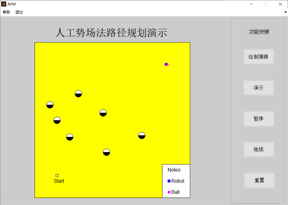
function state_Callback(hObject, eventdata, handles)
aa=['1.Enter the simulation interface and click <Drawing obstacles> Function keys draw obstacles in the work window' ...
char(10) '2.After drawing obstacles, right-click to finish drawing, and the cross cursor disappears to indicate completion' ...
char(10) '3.click <demonstration> Function key, which will be automatically demonstrated according to the reservation algorithm' ...
char(10) '4.click <suspend> Function key, the demonstration process will be suspended, click <continue> After the function key, the demonstration will continue from the pause position' char(10)...
'5.click <Reset> Function key, the simulation interface will return to the initial state and wait for operation again'];
msgbox(aa,'instructions');
% hObject handle to state (see GCBO)
% eventdata reserved - to be defined in a future version of MATLAB
% handles structure with handles and user data (see GUIDATA)
% --------------------------------------------------------------------
function about_Callback(hObject, eventdata, handles)
msgbox(' Beihang automation','about');
% hObject handle to about (see GCBO)
% eventdata reserved - to be defined in a future version of MATLAB
% handles structure with handles and user data (see GUIDATA)
% --------------------------------------------------------------------
function menu_Callback(hObject, eventdata, handles)
% hObject handle to out (see GCBO)
% eventdata reserved - to be defined in a future version of MATLAB
% handles structure with handles and user data (see GUIDATA)
% --------------------------------------------------------------------
function out_Callback(hObject, eventdata, handles)
selection=questdlg(['Exit the presentation window?'], ...
['sign out'],'Yes','No','Yes');%When the exit button is selected, a box asking whether to close is obtained
if strcmp(selection,'No')
return;
else
if strcmp(selection,'Yes')
clc; %When off is selected, all are cleared matla Enter all error messages on the face and close the image window at the same time
clear all;
delete(gcf);
else
return;
end
end
% hObject handle to out (see GCBO)
% eventdata reserved - to be defined in a future version of MATLAB
% handles structure with handles and user data (see GUIDATA)
Complete code or simulation consultation add QQ1575304183