1, Introduction

Grey Wolf Optimizer is inspired by the official account of Seyedali Mirjalili, and a meta heuristic algorithm was proposed in 2014. It mainly simulates the search for prey, encircling prey and attacking prey. After the source code pays attention to the public number, it returns to "wolf" or "GWO" to obtain.
inspire
Gray wolves belong to the canine family and are the top predators at the top of the food chain. Most of them like to live in groups, with an average of 5 ~ 12 per population. What is particularly interesting is that they have very strict social hierarchy, as shown in the figure below.

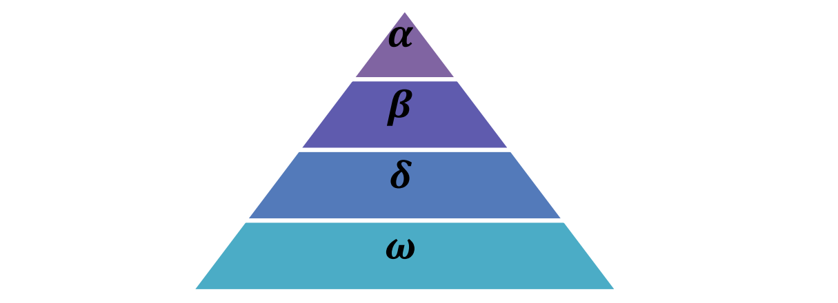
Figure 1 gray wolf stratification

The leading wolf (leader) is a male and a female, called alpha (personal understanding, so called because alpha is the first in the Greek subtitle, which is used to represent the front). Alpha wolves are mainly responsible for making decisions on hunting, sleeping place, getting up time, etc., and then transmitting the decision to the whole population. If the wolves hang their tails, they all agree. However, there will also be democratic behavior in the population, and alpha wolves will listen to other wolves in the population. Interestingly, alpha wolves are not necessarily the strongest members, but they are the best in managing the team. This shows that the organization and discipline of a wolf pack are far more important than its strength.

The second layer is beta. deta wolf is a subordinate wolf, which can be male or female. It is used to assist alpha wolf in decision-making or other population activities. When one of the alpha wolves dies or gets old, it is the best substitute for the alpha wolf. Beta wolves should follow alpha wolves, but they will also order other low-level wolves, so they play a connecting role.
At the bottom is omega wolf. They played the role of "scapegoat" (unfortunately), had to succumb to other leading wolves, and came last when eating. It seems that the omega wolf is not an important individual in the wolf pack, but once the omega wolf is lost, the whole wolf pack will face internal struggles and problems.
If a wolf is neither alpha, beta nor omega, it is called a subordinate wolf or delta wolf. Delta wolves must obey alpha and beta wolves, but will dominate omega wolves. Reconnaissance wolf, guard wolf, old wolf, predator wolf and guard wolf are all of this kind. Reconnaissance wolves are responsible for monitoring the boundary of the territory and warning the wolves in case of danger; Guarding wolves to protect and ensure the safety of wolves; Old wolves are experienced wolves who have retired from alpha or beta; Prey on wolves, help alpha and beta hunt and provide food for wolves; Taking care of wolves is responsible for taking care of the old, weak, sick and disabled in wolves.
In addition, group hunting is another interesting social behavior of gray wolves, which mainly includes the following stages:
Tracking, chasing and approaching prey;
Hunt, surround and harass prey until it stops moving;
Attack the prey.

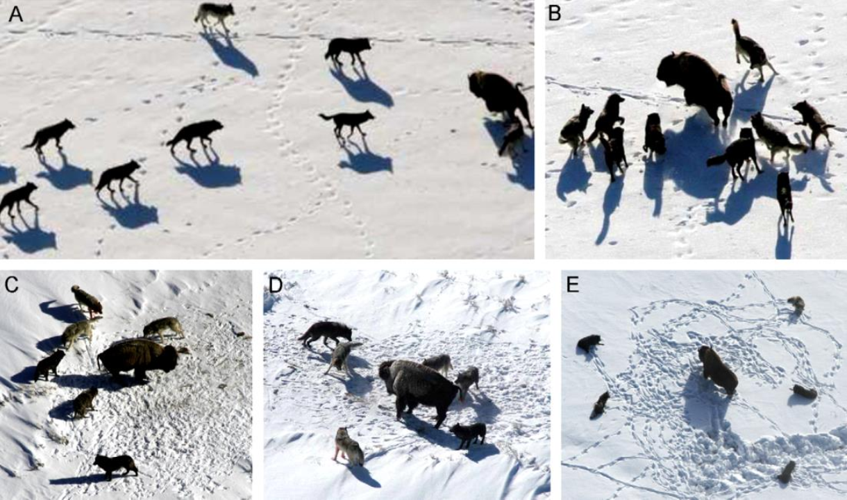
Figure 2 predation behavior of gray wolf: (A) chasing, approaching and tracking prey. (B-D) hunt, harass and surround prey. (E) Static state and attack
Mathematical model and algorithm
Firstly, the mathematical models of social hierarchy, tracking, encircling and attacking prey are given, and then a complete GWO algorithm is provided.
Social class
In order to model the social hierarchy of wolves mathematically when designing GWO, it is considered that the most appropriate solution is alpha( α \ alpha α)， Then the second and third optimal solutions are expressed as beta respectively( β \ beta β) And Delta( δ \ delta δ), The remaining solutions are assumed to be Omega( ω \ omega ω). In GWO, through α \ alpha α,β \ beta β and δ \ delta δ To guide predation (optimization), ω \ omega ω Listen to these three wolves.
Encircle predation
Gray wolves surround their prey when they prey. Use the following formula to express this behavior:
D ⃗ = ∣ C ⃗ ⋅ X p → ( t ) − X ⃗ ( t ) ∣ (1) \vec{D}=|\vec{C} \cdot \overrightarrow{X_{p}}(t)-\vec{X}(t)|\tag{1}D=∣C⋅Xp​​(t)−X(t)∣(1)
X ⃗ ( t + 1 ) = X p → ( t ) − A ⃗ ⋅ D ⃗ (2) \vec{X}(t+1)=\overrightarrow{X_{p}}(t)-\vec{A} \cdot \vec{D}\tag{2}X(t+1)=Xp​​(t)−A⋅D(2)
Where t tt represents the current number of iterations, a ⃗ \ vec{A}A and C ⃗ \ vec{C}C are coefficient vectors, X p → \ overrightarrow {x {P}} XP is the position vector of prey, and X ⃗ \ vec{X}X is the position vector of gray wolf.
Vectors a ⃗ \ vec{A}A and C ⃗ \ vec{C}C are calculated as follows:
A ⃗ = 2 a ⃗ ⋅ r ⃗ 1 − a ⃗ (3) \vec{A}=2 \vec{a} \cdot \vec{r}{1}-\vec{a}\tag{3}A=2a⋅r1​−a(3)
C ⃗ = 2 ⋅ r 2 → (4) \vec{C}=2 \cdot \overrightarrow{r{2}}\tag{4}C=2⋅r2​​(4)
The components of a ⃗ \ vec{a}a are linearly reduced from 2 to 0 in the iterative process, and R ⃗ 1 \vec{r}{1}r1 and r 2 → \ overrightarrow{r{2}}r2 are random vectors between [0,1].
In order to clearly reflect the effect of equations (1) and (2), the two-dimensional position vector and possible neighborhood are shown in Figure 3(a). It can be seen that the position (X,Y) (X,Y) (X,Y) of gray wolf can be updated according to the position of prey (X *, Y *) (X*,Y)(X *, Y *), by adjusting the values of a ⃗ \ vec{A}A and C ⃗ \ VEC {C}, You can reach different places relative to the current position around the optimal agent. For example, when a ⃗ = (0,1) \ VEC {a} = (0,1) a = (0,1) and C ⃗ = (1,1) \ VEC {C} = (1,1) C = (1,1), the new position of gray wolf is (X ∗− X,Y *) (X*-X,Y)(X ∗− X,Y *). The same is true in three-dimensional space. Note that the two figures here only show the case of a ⃗ = (0,1) \ VEC {a} = (0,1) a = (0,1) and C ⃗ = (1,1) \ VEC {C} = (1,1) C = (1,1), when the random vector r 1_ 1r1 # and r 2 r_2r2# when taking different values, the gray wolf can reach the position between any two points. At the same time, it is also noted that the value of AA will determine whether the gray wolf is close to or away from the prey, which will be explained in detail later.

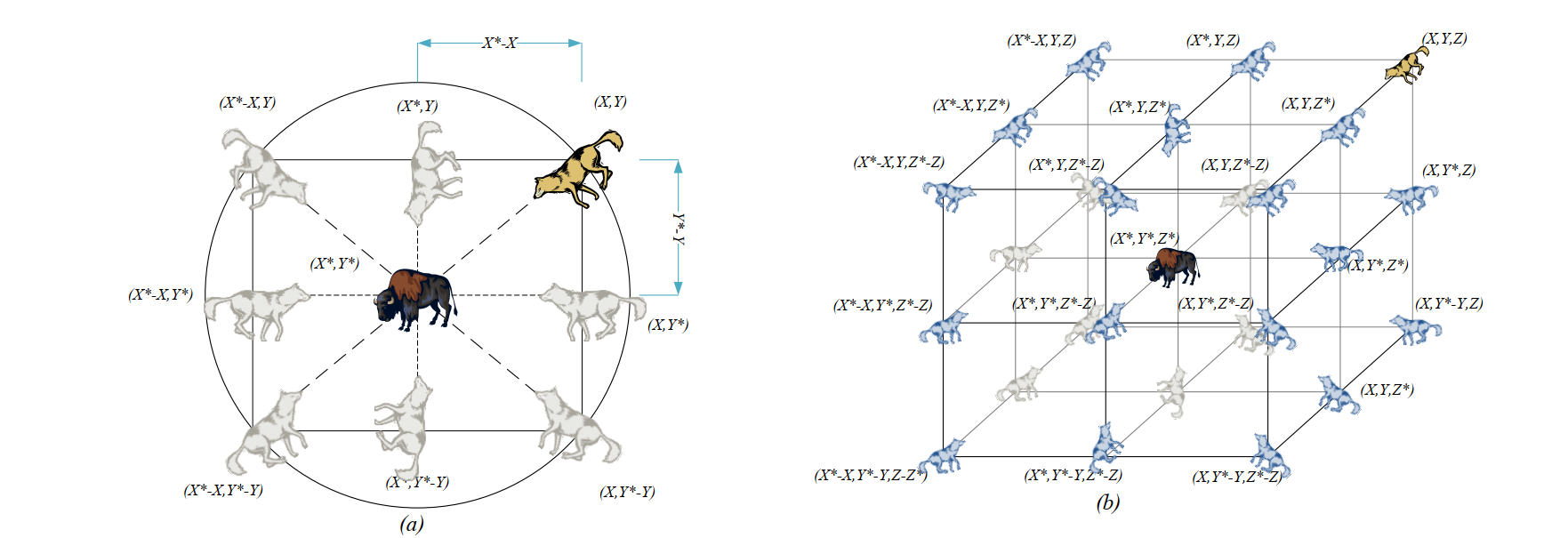
Figure 3 2D and 3D position vectors and their possible next positions
hunting
Gray wolves can identify the location of prey and surround them. Hunting is usually led by alpha wolves, and beta and delta wolves occasionally participate in hunting. However, in an abstract search space, we do not know the location of the best (prey). In order to mathematically simulate the hunting behavior of gray wolves, we assume that alpha (best candidate solution), beta and delta wolves have a better understanding of the potential location of prey. Therefore, we save the first three best solutions obtained so far and force other search agents (including omegas) to update their location according to the location of the best search agent. In this regard, the following formula is proposed:
D α → = ∣ C ⃗ 1 ⋅ X α → − X ⃗ ∣ , D β → = ∣ C ⃗ 2 ⋅ X β → − X ⃗ ∣ , D δ → = ∣ C 3 → ⋅ X δ → − X ⃗ ∣ (5) \overrightarrow{D_{\alpha}}=\left|\vec{C}{1} \cdot \overrightarrow{X{\alpha}}-\vec{X}\right|, \overrightarrow{D_{\beta}}=\left|\vec{C}{2} \cdot \overrightarrow{X{\beta}}-\vec{X}\right|, \overrightarrow{D_{\delta}}=|\overrightarrow{C_{3}} \cdot \overrightarrow{X_{\delta}}-\vec{X}|\tag{5}Dα​​=∣∣∣​C1​⋅Xα​​−X∣∣∣​,Dβ​​=∣∣∣​C2​⋅Xβ​​−X∣∣∣​,Dδ​​=∣C3​​⋅Xδ​​−X∣(5)

X 1 → = X α → − A 1 → ⋅ ( D α → ) , X 2 → = X β → − A 2 → ⋅ ( D β → ) , X 3 → = X δ → − A 3 → ⋅ ( D δ → ) 6 ) (() \overrightarrow{X_{1}}=\overrightarrow{X_{\alpha}}-\overrightarrow{A_{1}} \cdot(\overrightarrow{D_{\alpha}}), \overrightarrow{X_{2}}=\overrightarrow{X_{\beta}}-\overrightarrow{A_{2}} \cdot(\overrightarrow{D_{\beta}}), \overrightarrow{X_{3}}=\overrightarrow{X_{\delta}}-\overrightarrow{A_{3}} \cdot(\overrightarrow{D_{\delta}})\tag(6)X1​​=Xα​​−A1​​⋅(Dα​​),X2​​=Xβ​​−A2​​⋅(Dβ​​),X3​​=Xδ​​−A3​​⋅(Dδ​​)6)(()

X ⃗ ( t + 1 ) = X 1 → + X 2 → + X 3 → 3 (7) \vec{X}(t+1)=\frac{\overrightarrow{X_{1}}+\overrightarrow{X_{2}}+\overrightarrow{X_{3}}}{3}\tag{7}X(t+1)=3X1​​+X2​​+X3​​​(7)

Figure 4 shows how to update the proxy location according to alpha, beta and delta in 2D space. It can be seen that the final position will be a random position within the circle, which is defined by alpha, beta and delta. In other words, alpha, beta and delta wolves estimate the position of prey, while other wolves randomly update their position around the prey.

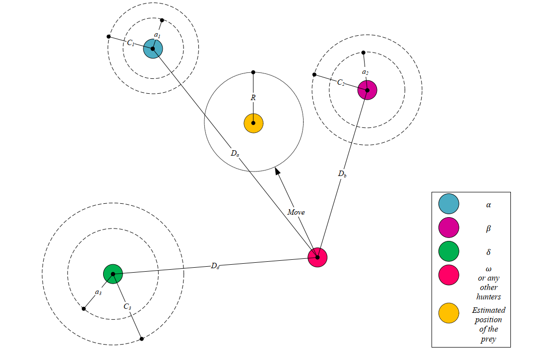
Figure 4 Schematic diagram of location update in GWO

Attack prey (use)
As mentioned above, when the prey stops moving, the gray wolf will attack it to complete the hunt. In order to model approaching prey, the value of A ⃗ \ VEC AA needs to be continuously reduced, and the fluctuation range of A ⃗ \ VEC AA will also be reduced. When A ⃗ ∈ [− 1,1] \ VEC A \ in [- 1,1] A ∈ [− 1,1], the next location of the search agent can be any location between the current location of the agent and the location of the prey. Figure 5(a) shows that when ∣ A ∣ < 1 | A | < 1 ∣ A ∣ < 1, gray wolves attack their prey.

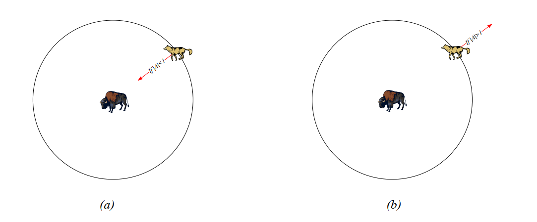
Figure 5 prey attack vs prey search

Search for prey (explore)
Gray wolves usually search according to the location of alpha, beta and delta wolves. They disperse to find prey, and then gather to attack prey. In order to model the dispersion mathematically, A ⃗ \ vec AA with random value greater than 1 or less than - 1 is used to force the search agent to deviate from the prey, so as to ensure the exploration. Figure 5(b) shows that when ∣ A ∣ > 1 | A | > 1 ∣ A ∣ > 1, gray wolves are forced to leave their prey in the hope of finding more suitable prey. Another factor supporting GWO exploration is C ⃗ \ vec CC. According to formula (4), the value range of C ⃗ \ vec CC is [0,2] [0,2] [0,2], which provides random weight for prey to randomly emphasize (c > 1) or weaken (C < 1)
The role of prey in defining the distance in equation (1). This helps GWO to show more random behavior in the whole optimization process, and is conducive to exploring and avoiding local optimization. C CC does not decrease linearly like A AA. C CC is specially required to provide random values at any time, so as to emphasize exploration not only in the initial iteration, but also in the final iteration.

C CC vector can also be considered as the influence of obstacles on approaching prey in nature. Generally speaking, obstacles in nature appear on the hunting path of wolves, which actually prevents them from approaching prey quickly and conveniently. This is what the vector C CC does. According to the location of the wolf, it can randomly give prey a weight, which makes the wolf's predation more difficult and distant, and vice versa.

GWO algorithm
In short, the search process starts with creating A random gray wolf population (candidate solution) in GWO algorithm. In the iterative process, alpha, beta and delta wolves estimate the possible location of prey. Each candidate solution updates its distance from the prey. In order to emphasize exploration and utilization respectively, the parameter a aa is reduced from 2 to 0. When ∣ A ⃗∣ > 1 | \ VEC A | > 1 ∣ A ∣ > 1, the candidate solution tends to deviate from the prey. When ∣ A ⃗∣ < 1 | \ VEC A | < 1 ∣ A ∣ < 1, the candidate solution converges to the prey. Finally, the GWO algorithm is terminated when the end condition is met. The pseudo code of GWO is as follows.

Initialize gray wolf population x I (I = 1, 2,..., n) x_ i(i=1,2,…,n)Xi​(i=1,2,…,n)

Initialize a, a, C, a, a, CA, a, C

Calculate the fitness value of each search agent

X α = X_{\alpha}=X α = best search agent

X β = X_{\beta}=X β = second best search agent

X δ = X_{\delta}=X δ = third best search agent

While (T < maximum number of iterations)

for each search agent

Update the location of the current agent according to equation (7)

end for

Update a, a, C, a, a, CA, a, C

Calculate fitness values for all search agents

Update x α X_{\alpha}X α ​,X β X_{\beta}X β ​,X δ X_{\delta}X δ ​

KaTeX parse error: Expected 'EOF', got '&' at position 1: &̲emsp; t=t+...

end while

return X α X_{\alpha}Xα​

Through the following points, we can understand how GWO solves the optimization problem in theory:

The proposed social hierarchy helps GWO to preserve the current optimal solution in the iterative process;
The proposed encirclement mechanism defines a circular neighborhood around the solution, which can be extended to higher dimensions as a hypersphere;
Hypersphere with different random radii for the auxiliary candidate solutions of random parameters AA and CC;
The proposed hunting method allows candidate solutions to determine the possible location of prey;
The adaptation of AAA and AAA ensures the exploration and utilization;
The adaptive values of parameters a AA and a AA make GWO realize a smooth transition between exploration and utilization;
With the decline of AA, half of the iterations are devoted to exploration (∣ A ∣ ≥ 1 |A | ≥ 1 ∣ A ∣ ≥ 1), and the other half is devoted to utilization (∣ A ∣ < 1 |A | < 1 ∣ A ∣ < 1);
GWO has only two main parameters to be adjusted (a aa and C CC).

2, Source code

 
clear all
clc
 
drawing_flag = 1;
 
TestProblem='UF1';
nVar=10;
 
fobj = cec09(TestProblem);
 
xrange = xboundary(TestProblem, nVar);
 
% Lower bound and upper bound
lb=xrange(:,1)';
ub=xrange(:,2)';
 
VarSize=[1 nVar];
 
GreyWolves_num=100;
MaxIt=1000;  % Maximum Number of Iterations
Archive_size=100;   % Repository Size
 
alpha=0.1;  % Grid Inflation Parameter
nGrid=10;   % Number of Grids per each Dimension
beta=4; %=4;    % Leader Selection Pressure Parameter
gamma=2;    % Extra (to be deleted) Repository Member Selection Pressure
 
% Initialization
 
GreyWolves=CreateEmptyParticle(GreyWolves_num);
 
 
for i=1:GreyWolves_num
    GreyWolves(i).Velocity=0;
    GreyWolves(i).Position=zeros(1,nVar);
    for j=1:nVar
        GreyWolves(i).Position(1,j)=unifrnd(lb(j),ub(j),1);
    end
    GreyWolves(i).Cost=fobj(GreyWolves(i).Position')';
    GreyWolves(i).Best.Position=GreyWolves(i).Position;
    GreyWolves(i).Best.Cost=GreyWolves(i).Cost;
end
 
GreyWolves=DetermineDomination(GreyWolves);
 
Archive=GetNonDominatedParticles(GreyWolves);
 
Archive_costs=GetCosts(Archive);
G=CreateHypercubes(Archive_costs,nGrid,alpha);
 
for i=1:numel(Archive)
    [Archive(i).GridIndex Archive(i).GridSubIndex]=GetGridIndex(Archive(i),G);
end
 
% MOGWO main loop
 
for it=1:MaxIt
    a=2-it*((2)/MaxIt);
    for i=1:GreyWolves_num
        
        clear rep2
        clear rep3
        
        % Choose the alpha, beta, and delta grey wolves
        Delta=SelectLeader(Archive,beta);
        Beta=SelectLeader(Archive,beta);
        Alpha=SelectLeader(Archive,beta);
        
        % If there are less than three solutions in the least crowded
        % hypercube, the second least crowded hypercube is also found
        % to choose other leaders from.
        if size(Archive,1)>1
            counter=0;
            for newi=1:size(Archive,1)
                if sum(Delta.Position~=Archive(newi).Position)~=0
                    counter=counter+1;
                    rep2(counter,1)=Archive(newi);
                end
            end
            Beta=SelectLeader(rep2,beta);
        end
        
        % This scenario is the same if the second least crowded hypercube
        % has one solution, so the delta leader should be chosen from the
        % third least crowded hypercube.
        if size(Archive,1)>2
            counter=0;
            for newi=1:size(rep2,1)
                if sum(Beta.Position~=rep2(newi).Position)~=0
                    counter=counter+1;
                    rep3(counter,1)=rep2(newi);
                end
            end
            Alpha=SelectLeader(rep3,beta);
        end
        
        % Eq.(3.4) in the paper
        c=2.*rand(1, nVar);
        % Eq.(3.1) in the paper
        D=abs(c.*Delta.Position-GreyWolves(i).Position);
        % Eq.(3.3) in the paper
        A=2.*a.*rand(1, nVar)-a;
        % Eq.(3.8) in the paper
        X1=Delta.Position-A.*abs(D);
        
        
        % Eq.(3.4) in the paper
        c=2.*rand(1, nVar);
        % Eq.(3.1) in the paper
        D=abs(c.*Beta.Position-GreyWolves(i).Position);
        % Eq.(3.3) in the paper
        A=2.*a.*rand()-a;
        % Eq.(3.9) in the paper
        X2=Beta.Position-A.*abs(D);
        
        
        % Eq.(3.4) in the paper
        c=2.*rand(1, nVar);
        % Eq.(3.1) in the paper
        D=abs(c.*Alpha.Position-GreyWolves(i).Position);
        % Eq.(3.3) in the paper
        A=2.*a.*rand()-a;
        % Eq.(3.10) in the paper
        X3=Alpha.Position-A.*abs(D);
        
        % Eq.(3.11) in the paper
        GreyWolves(i).Position=(X1+X2+X3)./3;
        
        % Boundary checking
        GreyWolves(i).Position=min(max(GreyWolves(i).Position,lb),ub);
        
        GreyWolves(i).Cost=fobj(GreyWolves(i).Position')';
    end
    
    GreyWolves=DetermineDomination(GreyWolves);
    non_dominated_wolves=GetNonDominatedParticles(GreyWolves);
    
    Archive=[Archive
        non_dominated_wolves];
    
    Archive=DetermineDomination(Archive);
    Archive=GetNonDominatedParticles(Archive);
    
    for i=1:numel(Archive)
        [Archive(i).GridIndex Archive(i).GridSubIndex]=GetGridIndex(Archive(i),G);
    end
    
    if numel(Archive)>Archive_size
        EXTRA=numel(Archive)-Archive_size;
        Archive=DeleteFromRep(Archive,EXTRA,gamma);
        
        Archive_costs=GetCosts(Archive);
        G=CreateHypercubes(Archive_costs,nGrid,alpha);
        
    end
    
    disp(['In iteration ' num2str(it) ': Number of solutions in the archive = ' num2str(numel(Archive))]);
    save results
    
    % Results
    
    costs=GetCosts(GreyWolves);
    Archive_costs=GetCosts(Archive);
    
    if drawing_flag==1
        hold off
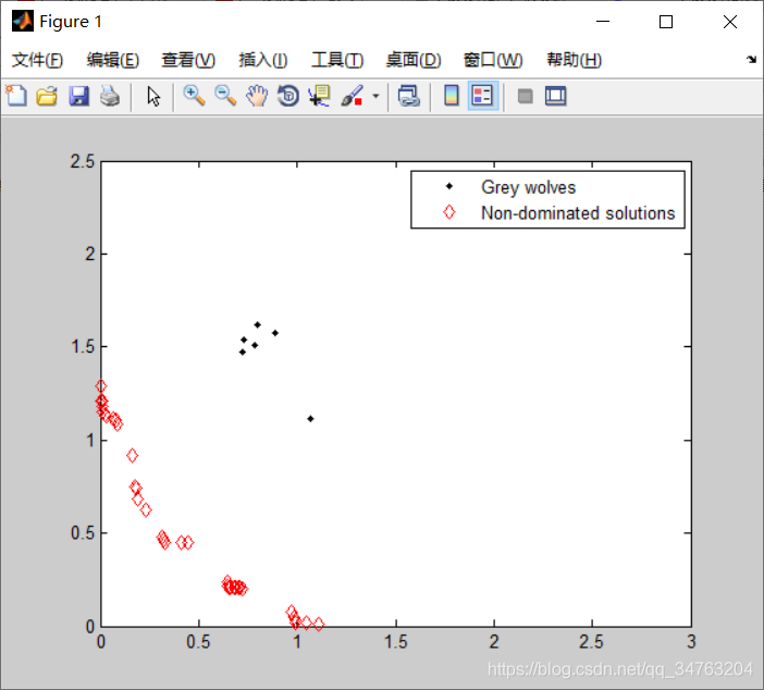
        plot(costs(1,:),costs(2,:),'k.');
        hold on
        plot(Archive_costs(1,:),Archive_costs(2,:),'rd');
        legend('Grey wolves','Non-dominated solutions');
        drawnow
    end
    
end
 
 

3, Operation results

4, Remarks

Version: 2014a