1, Mathematical representation of fault information

In the figure above, K represents the circuit breaker, and each circuit breaker has an FTU device, which can feed back whether the circuit breaker switch is overcurrent. It is used to represent the uploaded fault information, which reflects whether the fault current flows at each section switch (if there is fault current, it is 1, otherwise it is 0). Namely:

 

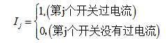
Because the information uploaded by FTU can be divided into fault information and fault-free information, and it can only be fault and fault-free for segmented sections, we can use binary coding rules to mathematically model the fault location problem of distribution network. Taking the radial distribution network shown in the figure above as an example, the system has 12 section switches. We can use a string of 12 bit binary code to represent the upload information of FTU as the input of the program. 1 represents that the corresponding switch has overcurrent information and 0 represents that the corresponding switch has no overcurrent information. At the same time, another string of 12 bit binary code is used as the output of the program to represent the failure of the corresponding feeder section and no failure.

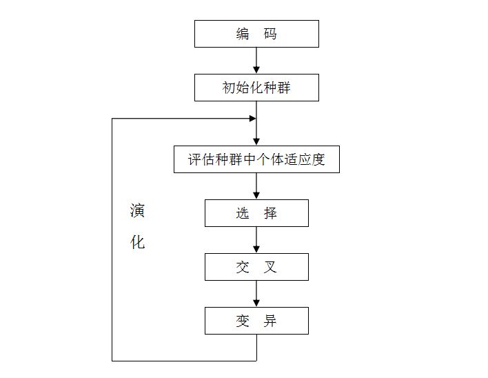
Genetic algorithm starts with a population representing the possible potential solution set of the problem, and a population is composed of a certain number of individuals encoded by gene s. Each individual is actually an entity with a characteristic chromosome.

Chromosome is the main carrier of genetic material, that is, the collection of multiple genes. Its internal performance (i.e. genotype) is a certain gene combination, which determines the external performance of individual shape. For example, the feature of black hair is determined by a certain gene combination in the chromosome that controls this feature. Therefore, at the beginning, it is necessary to realize the mapping from phenotype to genotype, that is, coding. Because the work of imitating gene coding is very complex, we often simplify it, such as binary coding.

After the generation of the first generation population, according to the principle of survival of the fittest and survival of the fittest, generation evolves to produce better and better approximate solutions. In each generation, individuals are selected according to the fitness of individuals in the problem domain, With the help of genetic operators of natural genetics, the population representing the new solution set is generated by combining crossover and mutation.

This process will lead to the later generation population like natural evolution, which is more suitable for the environment than the previous generation. After decoding, the optimal individual in the last generation population can be used as the approximate optimal solution of the problem.

2, Genetic algorithm process diagram

 

3, Constructing distribution network fault location evaluation function

Based on the principle that the deviation between the information corresponding to the actual state of each feeder section to be calculated and the actual uploaded fault information shall be the smallest, the following evaluation function is constructed:

 

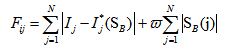
The value of the expression is the fitness value corresponding to each potential solution. The smaller the value, the better the solution. Therefore, the evaluation function should take the minimum value.

Where:It is the fault information uploaded by the j th switch FTU. If the value is 1, it is considered that the fault current flows through the switch, and if it is 0, it does not flow;Is the expected state of each switch node. If the switch flows fault current, the expected state is 1. On the contrary, the expected state is 0, and the expression is a function of each section state. N is the total number of feeder sections in the distribution network,Is the status of each equipment in the distribution network. If it is 1, it indicates equipment failure. If it is 0, the equipment is normal.Represents a weight coefficient multiplied by the number of faulty equipment,. It is a weight coefficient set according to the concept of "minimum set" in fault diagnosis theory, and the value range is between and 1, indicating that the fewer the number of fault intervals, the better the solution and avoid false diagnosis. In this paper, the weight coefficient is 0.5.

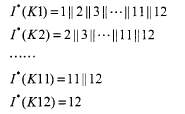
4, Find the expected function

For different networks, the expression of expectation function is different, which can not be expressed in a unified format. Only the above example is used to illustrate how to obtain the expected function.

In the radial distribution network, the fault of any section will lead to the fault overcurrent of its upstream switch. This is the principle of finding the expected function. Assuming a fault occurs at feeder section 6 in Figure 1, the sectional switches K1, K2, K3 and K6 will have overcurrent. If a fault occurs at feeder section 11, K1, K2, K3, K6 and K10 will have overcurrent. By analogy, we can get the expected function of each section switch:

 
%Using improved genetic algorithm and coding based on ring network, it is easy to produce feasible solution (meet the radial constraint of distribution network)
%be used for IEEE33 The fitness of node distribution network fault recovery is to calculate the network loss and operation times
%The choice is roulette
%The shift operation and mutation operation will not produce infeasible solutions and do not need to be tested
 
clear;
clc;
tic
%Based on the coding strategy of ring network, the common branch only needs to be placed in one ring network, and switch 1 does not need coding (always closed)
loop1=[2,3,4,5,18,19,20,33];
loop2=[22,23,24,25,26,27,28,37];
loop3=[8,9,10,11,21,35];
loop4=[6,7,15,16,17,29,30,31,32,36];
loop5=[12,13,14,34];
%Determine the fault branch(with txt File form input)
% txtpath='breaker.txt';%File pathname
bb=36;
%Store initial switch set
population1=[1,1,1,1,1,1,1,0,1,1,1,1,1,1,1,0,1,1,1,1,1,0,1,1,1,1,1,1,1,1,1,0,1,1,1,0]; 
%Population size
popsize=50;
%Gene block coding length
%chromlength=5;
%Shift probability
pc = 0.6;
%Variation probability
pm = 0.001;
%Initial population
pop = initpop(popsize,bb);
%initialization x,y(Store the optimal solution under each iteration)
x=zeros(1,50);
y=zeros(50,size(pop,2));
%Calculate fitness value
fitvalue = cal_fitvalue(pop);     
for i = 1:50  %50 Second iteration
    %Select operation
    newpop = selection(pop,fitvalue);
    %Shift operation
    newpop = moveposition(newpop,pc,bb);
    %Mutation operation
    newpop = mutation(newpop,pm,bb);
    %Renewal population
    pop = newpop;
    %Calculate the fitness value and find the optimal solution
    fitvalue = cal_fitvalue(pop);
    [bestindividual,bestfit] = best(pop,fitvalue);  
    %ws(i)=powerflow(transform(bestindividual)); %Record the actual network loss
    %cz(i)=sum(xor(bestindividual,population1))-1; %Record actual operation times
    x(i)=bestfit;
    y(i,:)=bestindividual;
end
[bestfit1,index]=max(x);
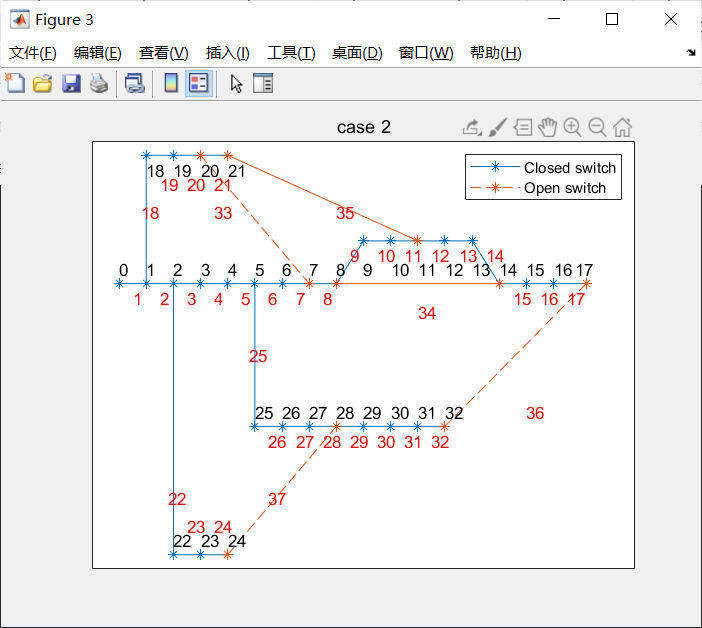
%Show initial topology
figure
show_tuopu(population1);
saveas(gca,'tuopu1.jpg'); %Save topology output in picture format
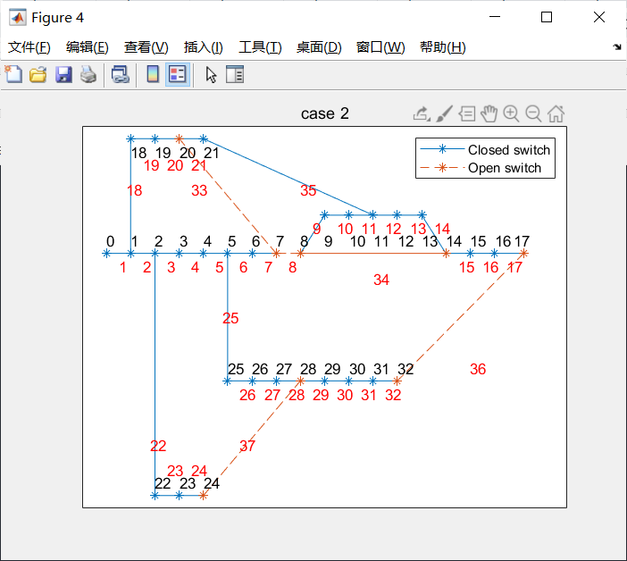
%Display the distribution network topology corresponding to the maximum fitness value
figure
show_tuopu(y(index,:));
saveas(gca,'tuopu.jpg'); %Save topology output in picture format
%Output the best fitness value under each iteration number
x;
bestfit1;
y(index,:);
%Output specific operation switch
[openkg,closekg] = judge_kg(y(index,:),bb); %Find out the switches that need to be turned off and closed under the optimal topology
fid=fopen('openkg.txt','wt');  %Convert the calculation results to txt Output as file
fprintf(fid,'%g\n',openkg);
fclose(fid);
fid=fopen('closekg.txt','wt');  %Convert the calculation results to txt Output as file
fprintf(fid,'%g\n',closekg);
fclose(fid);
%Output the network speed and operation times of distribution network corresponding to the best topology
ws = powerflow(transform(y(index,:)))
cz = sum(xor(y(index,:),population1))-1
%result=[ws;cz];
fid=fopen('ws.txt','wt');  %Convert the calculation results to txt Output as file
fprintf(fid,'%g\n',ws);
fclose(fid);
fid=fopen('cz.txt','wt');  %Convert the calculation results to txt Output as file
fprintf(fid,'%g\n',cz);
fclose(fid);
%Node voltage of output power flow calculation
[node,u,delt]=powerflow_V(transform(y(index,:)));
nodevoltage=[node',u',delt'];
fid=fopen('nodevoltage.txt','wt');  %Convert the calculation results to txt Output as file
[m,n]=size(nodevoltage);
for i=1:m
   for j=1:n
      if j==n
          fprintf(fid,'%g\n',nodevoltage(i,j));
      else
          fprintf(fid,'%g\t',nodevoltage(i,j));
      end
   end
end
fclose(fid);
%Branch current of output power flow calculation
[branch,p,q]=powerflow_S(transform(y(index,:)));
branchflow=[branch',p',q']
fid=fopen('branchflow.txt','wt');  %Convert the calculation results to txt Output as file
[m,n]=size(branchflow);
for i=1:m
   for j=1:n
      if j==n
          fprintf(fid,'%g\n',branchflow(i,j));
      else
          fprintf(fid,'%g\t',branchflow(i,j));
      end
   end
end
fclose(fid);
toc
 

Complete code or write on behalf of QQ1575304183