Using MATLAB to draw a better vector diagram

The basic data unit of MATLAB is matrix. Using MATLAB, it is convenient to draw vector distribution map, such as the sampling data of air flow; Gradient of function; The normal vector of the surface, and so on. Matlab's built-in quiver and quiver3 functions can meet this demand, but the arrow type of the arrow is relatively simple. The main purpose here is to further draw a better vector graph.

MATLAB vector graph function quiver

The built-in functions of quiver and quiver3 in Matlab can draw simple vector graphs. The basic syntax is Quiver (x, Y, U, V) and quiver3 (x, Y, Z, U, V, w). Arrows with directional components U and V are drawn on the Cartesian coordinates specified by X and Y. Adjust the length of the arrow and set syntax references such as linetype, mark and color MATLAB Help Center.
Example 1 (source: MATLAB Help Center)
Draw function z = x e − x 2 − y 2 z=xe^{-x^2-y^2} Z = gradient and contour of Xe − x2 − y2.
First, create an equally spaced x x x and y y A grid of y values. Use them to calculate z z z. Then, by specifying the spacing between points, the z z The gradient of z.
Code slice

spacing = 0.2;
[X,Y] = meshgrid(-2:spacing:2);
Z = X.*exp(-X.^2 - Y.^2);
[DX,DY] = gradient(Z,spacing);

Displays the gradient vector as an arrow diagram. Then, the contour lines are displayed in the same coordinate area. Adjust the display so that the gradient vector is perpendicular to the contour by calling axis equal.
Code slice

quiver(X,Y,DX,DY)
hold on
contour(X,Y,Z)
axis equal
hold off

Example 2 (source: MATLAB Help Center)
Draw perpendicular to function z = x e − x 2 − y 2 z=xe^{-x^2-y^2} The vector of the surface defined by z=xe − x2 − y2.
First, create an equally spaced x x x and y y A grid of y values. Use them to calculate z z z. Then, find the normal vector.
Code slice

[X,Y] = meshgrid(-2:0.25:2,-1:0.2:1);
Z = X.*exp(-X.^2 - Y.^2);
[U,V,W] = surfnorm(X,Y,Z);

Displays the vector as a three-dimensional arrow diagram. Then, the surface is displayed in the same coordinate area. Adjust the display by calling axis equal so that the vector appears perpendicular to the surface.
Code slice

quiver3(X,Y,Z,U,V,W)
hold on
surf(X,Y,Z)
axis equal

Draw 3D arrow with MATLAB

Here, we first write a simple function to draw a 3D arrow, input the position (a,b,c) and orientation (alpha,beta,gamma) of the arrow, return the 3D arrow in the coordinate area, and control the size, shape, color and other parameters of the arrow. The arrow consists of four parts: conical side + cylindrical side + conical bottom + conical bottom. Therefore, we set four parts S1, S2, S3 and S4 for the output.
The function expression is as follows
Code slice

function [s1,s2,s3,s4] = quiver_Refine(a,b,c,alpha,beta,gamma)
...
end

Drawing circular hammer with MATLAB

First draw the side and bottom of the cone:
Code slice

% Cone
r1 = 0:0.01:0.25; % The cone radius
h1 = 0.5;         % The cone height
% The cone top position
a1 = a;    
b1 = b;
c1 = 0.5;
% Generate cone data
[u,v,w] = cylinder(r1,50);
u = u+a1;
v = v+b1;
w = -w*h1+c1+c;
% Cone botton
t1 = (0:0.04:2)*pi;
r = max(r1(:));
xc = a1;
yc = b1;
zc = c1-h1+c;
% Generate cone botton data
x1 = xc + cos(t1)*r;
y1 = yc + sin(t1)*r;
[m,n] = size(x1);
z1 = repmat(zc,m,n);

In the back, the surf function is used to draw the side of the round hammer; Drawing conical bottom with fill3

Drawing cylinder with MATLAB

Then draw the side of the cylinder and the bottom of the cylinder, and the position of the top of the cylinder is connected to the bottom of the cone:
Code slice

% Cylinder
r2 = 0.1; % The cylinder radius
h2 = 0.5; % The cylinder height
% The cylinder top position
a2 = a1;
b2 = b1;
c2 = c1-h1;
% Generate cylinder data
[x,y,z] = cylinder(r2,50);
x = x+a2;
y = y+b2;
z = -z*h2+c2+c;
% Cylinder botton
t2 = (0:0.04:2)*pi;
r = r2;
xc = a2;
yc = b2;
zc = c2-h2+c;
% Generate cylinder botton data
x2 = xc + cos(t2)*r;
y2 = yc + sin(t2)*r;
[m,n] = size(x2);
z2 = repmat(zc,m,n);

Using surf function to draw the side of circular hammer cylinder; Drawing the bottom surface of conical cylinder with fill3
Code slice

%plot
s1 = surf(u,v,w,'Facecolor',color,'Edgecolor','none');
s2 = surf(x,y,z,'Facecolor',color,'Edgecolor','none');
s3 = fill3(x1,y1,z1,color,'Edgecolor','none');
s4 = fill3(x2,y2,z2,color,'Edgecolor','none');

A complete arrow can be drawn here. The position is determined by (a, b, c). At this time, the direction is along by default + z +z +The z direction is the (0, 0, 1) direction, and the color is determined by the color variable.

Arrow direction and color control

The direction control of the arrow is realized by the rotate function.
Code slice

% Rotate arrow
zc = (c1+zc)/2;
hold on
origin = [xc,yc,zc];
theta2 = acos(gamma./sqrt(alpha.^2 + beta.^2 + gamma.^2));
if beta^2 + alpha^2 == 0
    direct = [0 1 0];
else
    direct = [-beta,alpha,0];
end

Then, coordinate transformation can be carried out for the four components of the previous arrow
Code slice

if theta2 ~= 0
rotate(s1,direct,rad2deg(theta2),origin);
rotate(s2,direct,rad2deg(theta2),origin);
rotate(s3,direct,rad2deg(theta2),origin);
rotate(s4,direct,rad2deg(theta2),origin);
end

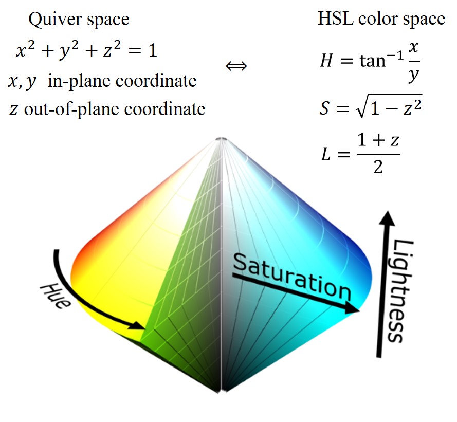
The color control of the arrow can customize the composition of the color variable. For example, here the arrow is in x y xy Azimuth in xy plane ϕ \phi ϕ Binding with color ring colorwheel, polar angle θ \theta θ Bound to brightness intensity. Color is in HSL space H S L HSL HSL three components and α \alpha α, β \beta β, γ \gamma γ corresponding

Code slice

% control quiver color using HSL
H = atan2(beta,alpha);
% Get the atan2 space in 0 ~ 2*pi
if H < 0
    H = 2*pi+H;
end

% rotate clockwisely
H = H + theta/180*pi;
if H < 0
    H = H + 2*pi;
elseif H >2*pi
    H = H - 2*pi;
end

S = sqrt(1-gamma^2);
I = (gamma+1)/2;

% change HSL to RGB 
idx = find((0 <= H)&(H < 2*pi/3));
B(idx) = I(idx).*(1-S(idx));
R(idx) = I(idx).*(1+S(idx).*cos(H(idx))./cos(pi/3-H(idx)));
G(idx) = 3*I(idx)-(B(idx)+R(idx));

idx = find((2*pi/3 <= H)&(H < 4*pi/3));
R(idx) = I(idx).*(1-S(idx));
G(idx) = I(idx).*(1+S(idx).*cos(H(idx)-2*pi/3)./cos(pi-H(idx)));
B(idx) = 3*I(idx)-(G(idx)+R(idx));

idx = find((4*pi/3 <= H)&(H <= 2*pi));
G(idx) = I(idx).*(1-S(idx));
B(idx) = I(idx).*(1+S(idx).*cos(H(idx)-4*pi/3)./cos(5*pi/3-H(idx)));
R(idx) = 3*I(idx)-(G(idx)+B(idx));

color = [R G B];
color(isnan(color)) = 0;
% Get color in the right range
for i=1:3
    color(i)=max(min(color(i),1),0);
end

Here, because the color in MATLAB is interpreted as RGB, it needs to be transformed from HSL space to RGB space. In fact, it can also be realized through hsv2rgb function.

Light parameter adjustment

MATLAB has a complete set of lighting parameter settings. The functions provided by graphics are similar to those of cameras with zoom lens, which can control the scene view created by MATLAB. For details, please refer to Camera graphics terminology . The commands provided by the MATLAB graphics environment allow you to place light sources and adjust the characteristics of objects that reflect light. For details, see Lighting overview . Here we can control the illumination to make the arrow look more three-dimensional.
Code slice

% lighting settings
axis equal 
camlight('left');
lighting phong 
view(3)

New quilver effect display

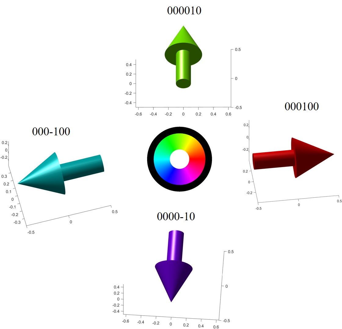
With the above settings, we can debug our own quiver_Refine function:
quiver_Refine(0,0,0,1,0,0);quiver_Refine(0,0,0,-1,0,0);
quiver_Refine(0,0,0,0,1,0);quiver_Refine(0,0,0,0,-1,0);

Effect display after position / direction matrix input

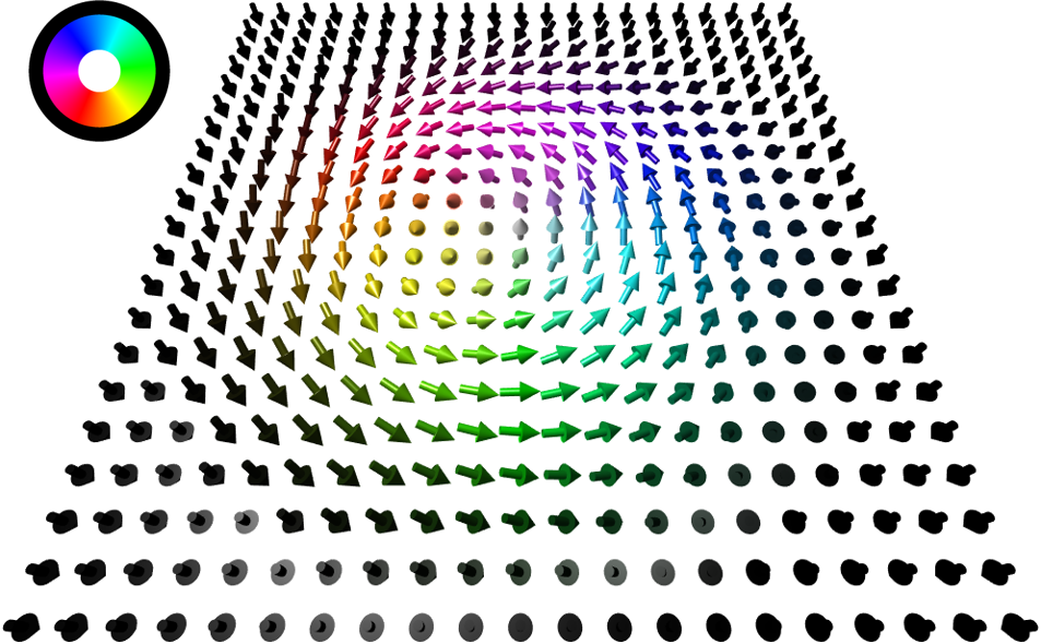
Current quiver_ The refine version only supports the input of data at a single location. It needs to use the for loop to call continuously, and the running speed is slow. However, the final result looks a little better than the original quiver function. Here, take Bloch skyrmion as an example. Turn Colorwheel 120 ° clockwise and dye quiver. Well, it's pretty good.