Pytorch: Overview of target detection networks, indicator calculation and use of pre-training networks
Copyright: Jingmin Wei, Pattern Recognition and Intelligent System, School of Artificial and Intelligence, Huazhong University of Science and Technology
This tutorial is not commercial and is only for learning and reference exchange. If you need to reproduce it, please contact me.
Reference
RCNN(Regions with CNN Features)
SSD(Single Shot MultiBox Detector)
Pytorch Object Detection in Deep Learning
Note: The datasets used in the object detection tutorial are mainly ImageNet, COCO, PASCAL VOC, which are three commonly used target detection datasets. Please consult the data for download and use of related datasets.
import numpy as np
import sys
from PIL import Image, ImageDraw, ImageFont
import matplotlib.pyplot as plt
import os

import torchvision
import torch
import torchvision.transforms as transforms
Object Detection Technology
In many technical fields of computer vision, object detection is a very basic task. Image segmentation, object tracking, key point detection and so on are usually dependent on object detection. In addition, because the number, size and posture of objects in each image are different, i.e. unstructured output, which is very different from image classification, objects are often blocked and truncated, and object detection technology is very challenging. Since its birth, it has been one of the most focused areas of researchers.
Object detection technology, usually refers to the detection of the location and corresponding categories of objects in an image. For people in the diagram, we require detector output 5 5 Five quantities: object category, x min , y min , x max , x max x_{\min}, y_{\min},x_{\max},x_{\max} xmin, ymin, xmax, xmax Of course, for a border, the detector can also output the form of center point and width and height, which are equivalent.
In computer vision, image classification, object detection and image segmentation are the foundation and the most rapid development at present. 3 3 Three areas.
Image Classification: Input images often contain only one object to determine what object each image is. It is an image-level task. It is relatively simple and develops the fastest.
Object detection: There are often many objects in the input image to determine the location and category of objects. It is a very core task in computer vision.
Image segmentation: Input is similar to object detection, but it is important to determine which category each pixel belongs to and which category belongs to at the pixel level. There are many links between image segmentation and object detection tasks, and models can also learn from each other.
Traditional way
Before using in-depth learning to do object detection, traditional algorithms usually classify object detection into area selection, feature extraction and feature classification. 3 3 Three stages.
area field choose take → special sign carry take → special sign branch class Zone Selection\rightarrow Feature Extractionrightarrow Feature Classification Region Selection_Feature Extraction_Feature Classification
- Region selection: Select the position of the object that may appear in the image first. Because the position and size of the object are not fixed, traditional algorithms usually use Sliding Windows algorithm, but this algorithm has a lot of redundant boxes and high computational complexity.
- Feature extraction: After obtaining the position of an object, the feature extraction is usually performed using a well-designed extractor, such as SIFT and HOG. Because the extractor contains fewer parameters and the robustness of the artificial design is low, the quality of feature extraction is not high.
- Feature Classification: Finally, the features obtained from the previous step are classified, usually using classifiers such as SVM, AdaBoost.
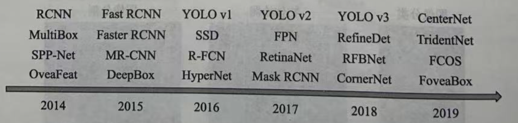
Target Detection Network
The development of object detection in the era of deep learning is illustrated in the figure. A large number of parameters of deep neural network can improve
Take out the features with better robustness and semantics, and classifier performance is better.
2014
2014
The 2014 CNN (Regions with CNN features) is a classic work of using deep learning to achieve object detection, which starts the prelude of deep learning to do object detection.
R-CNN
Reference article: Rich feature hierarchies for accurate object detection and semantic segmentation
Its main algorithms are divided into 4 4 Four phases:
-
Candidate Region Generation: Each image is generated using the Selective Search method 1000 − 2000 1000-2000 1000_2000 candidate regions.
-
Feature extraction: For each generated candidate area, normalize to a uniform size, and use deep convolution network to extract the characteristics of the candidate area.
-
Category judgment: CNN features are fed into each class of SVM classifiers to determine whether candidate regions belong to this class.
-
Location Refinement: Use regressor surprises to correct candidate box positions.
On the basis of RCNN, 2015 2015 Fast RCNN implemented end-to-end detection and convolution sharing in 2015.
Fast R-CNN
Reference article: Faster R-CNN: Towards Real-Time Object Detection with Region Proposal Networks
Fast R-CNN is the foundational work of the two-stage method. The proposed RPN network replaces the Selecctive Search algorithm to enable the detection task to be completed end-to-end by the neural network.
The specific method is to place the RPN after the last convolution layer, and then train the RPN directly to get the candidate regions. RPN network is characterized by extracting candidate boxes by sliding windows, sliding windows on feature mapping, and generating each sliding window position 9 9 Nine candidate windows with different scales and widths and heights to extract corresponding 9 9 Features of nine candidate windows for target classification and border regression.
Target classification only needs to distinguish if the feature in the candidate box is foreground or Beijing, and similar to Fast R-CNN, border regression determines a more precise target location.
Faster RCNN then proposed the epochal idea of Anchor, pushing object detection to its first peak. stay 2016 2016 In 2016, YOLO v1 implemented the first-order detection of Anchor-Free and SSD implemented the first-order detection of multi-feature maps. These two algorithms also have a profound impact on subsequent physical detection, which will be described in detail in a chapter in subsequent tutorials.
YOLO
Reference article: You Only Look Once: Unified, Real-Time Object Detection
YOLO(You Only Look Once) is a classical single target detection algorithm, which integrates target area prediction and target category prediction into a single neural network model to detect and identify targets quickly with high accuracy. The main advantages of YOLO are fast detection speed, global processing, relatively few background errors, and good generalization performance. However, due to the limitations of YOLO design, it is difficult to detect small targets.
The algorithm flow is as follows:
First divide the image into S × S S\times S S × S grids, and then on each grid, a deep convolution network is used to give the class judgment described by its objects (images are represented by different colors), and on the basis of the grid, B borders (boxes) are generated, with each border predicted 5 5 Five regression values, of which the first 4 4 Four values represent the position of the border, and the fifth value represents the probability that the border contains an object and the accuracy of the position. Finally, the final prediction box is obtained by NMS non-maximum suppression filtering.
stay 2017 2017 In 2017, FPN implemented a better feature extraction network using feature pyramids, while Mask RCNN improved the performance of object detection while implementing instance segmentation. Get into 2018 2018 After 2018, there are more algorithms for object detection, such as CornerNet, TidentNet with multiple receptive field branches, CenterNet with center points, etc.
In the object detection algorithm, the border of an object starts from nothing, and the change of the border reflects to some extent whether the detection is first or second order.
- Second-order: Typical algorithms such as RCNN, Faster RCNN focus on finding the location of an object in the first stage, get a recommendation box to ensure sufficient Recall, and then on classifying the recommendation boxes to find more accurate locations in the second stage. Second-order algorithms are usually more accurate but slower. Of course, there are more order algorithms such as Cascade RCNN.
- First-order: The first-order algorithm combines two phases of the second-order algorithm, and finds the location and category of objects in one phase. The method is usually simpler. It relies on the excellent network experience of feature fusion, (Focal Loss, etc.), which is generally faster than the second-order network, but with some loss of accuracy. Typical algorithms such as SSD, YOLO, RetinaNet, etc.
Anchor is an epoch-making idea that first appeared in Faster RCNN. Essentially, it is a series of priori boxes of varying sizes, widths and heights, which are evenly distributed on the feature map and used to predict the categories of these Anchors and their offsets from the borders of real objects. Anchor is equivalent to providing a ladder for object detection, so that the detector can not directly predict objects from scratch. The accuracy is often higher. The common algorithms are Faster RCNN, SSD, YOLO v2, etc.
Of course, there are also some anchorless algorithms with more diverse ideas, such as YOLO v1, which can directly predict the location of the border by its features. Recently, there have been many algorithms that rely on key points to detect objects, such as CornerNet, CenterNet, and so on.
Technology Application Areas
Due to the rapid improvement of detection performance, object detection is also an area of in-depth learning in which large-scale applications in the industry have been achieved. 5 5 Five widely used areas.
- Security: Under the influence of in-depth learning, the security field has achieved rapid development and landing in recent years. For example, the well-known face recognition technology has mature applications at traffic junctions, stations and so on. In addition, the detection of pedestrians and vehicles is a particularly important part of the security of smart cities. In the field of security, there is a great trend to incorporate detection technology into the camera to form a smart camera, which is best known by many companies such as Haikangwei and Horizon.
- Auto-driving: In the perception task of auto-driving, the detection of pedestrians, vehicles and other obstacles is particularly important. Because of the safety involved in driving, auto-driving requires a very high performance of detectors, especially the recall rate. Auto-driving is also known as the "Everest" of artificial intelligence applications. In addition, since vehicles need to obtain the three-dimensional position of obstacles relative to themselves, a lot of post-processing perception modules are usually added after the detector.
- Robots: In the automatic sorting of industrial robots, the system needs to identify the various parts to be sorted, which is a very typical application field of robots. In addition, mobile intelligent robots need to detect obstacles in the environment at all times to achieve safe obstacle avoidance and navigation. In a broad sense, auto-driving vehicles can also be viewed as a form of robots.
- Search recommendation: Object detection is everywhere in the major application platforms of Internet companies. For example, for image filtering, filtering, recommendation, and watermarking containing specific objects, more rich applications, such as dithering, are added based on face and pedestrian detection.
- Medical Diagnosis: Based on artificial intelligence and large data, medical diagnosis is also ushering in a new spring. With object detection technology, we can diagnose specific joints and diseases in CT, MR and other medical images more accurately and quickly.
evaluating indicator
For a detector, we need to formulate rules to evaluate it and select the desired detector. For image classification tasks, because the output is a very simple image category, it is easy to measure by judging the number of correctly classified images.
Intersection of Union(IoU)
The output of the object detection model is unstructured, and the number, location, size of the output object are not known beforehand, so the evaluation algorithm for object detection is slightly more complex. For a specific object, we can judge the quality of the detection by how well the prediction box fits the real box, usually using the IoU(Intersection of Union) to quantify the fit.
The IoU is calculated as shown in the figure below, using the ratio of the intersection and union of the two borders to obtain the IoU, as shown in the formula below. Obviously, the interval for loU is [ 0 , 1 ] [0,1] [0,1], the larger the IoU value, the better the two boxes coincide.
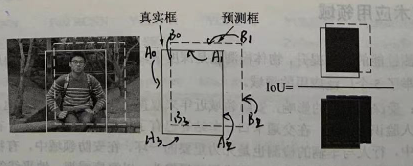
I o U A , B = S A ∩ S B S A ∪ S B IoU_{A,B}=\frac{S_A\cap S_B}{S_A\cup S_B} IoUA,B=SA∪SBSA∩SB
Code makes it easy to compute IoU:
def IoU(boxA, boxB):
    # Calculate the values of the top, bottom, left, and right sides of the coincident part
    left_max = max(boxA[0], boxB[0]) # X_ Larger x-coordinates in the left
    top_max = max(boxA[1], boxB[1]) # Y_ Larger y-coordinates in top
    right_min = min(boxA[2], boxB[2]) # X_ Smaller x-coordinates in right
    bottom_min = min(boxA[3], boxB[3]) # Y_ Smaller y-coordinates in bottom
    # Calculate coincident area
    inter = max(0, right_min-left_max) * max(0, bottom_min-top_max)
    # Calculate the area of two boxes
    SA = (boxA[2] - boxA[0]) * (boxA[3] - boxA[1])
    SB = (boxB[2] - boxB[0]) * (boxB[3] - boxB[1])
    # Calculate the area of all areas
    union = SA + SB - inter
    iou = inter / union
    return iou
For IoU, we usually pick a Fujian value, such as 0.5 0.5 0.5 to determine if the prediction box is correct or incorrect. When the IoU of two boxes is greater than 0.5 0.5 At 0.5, we think it's a valid check, otherwise it's an invalid match.
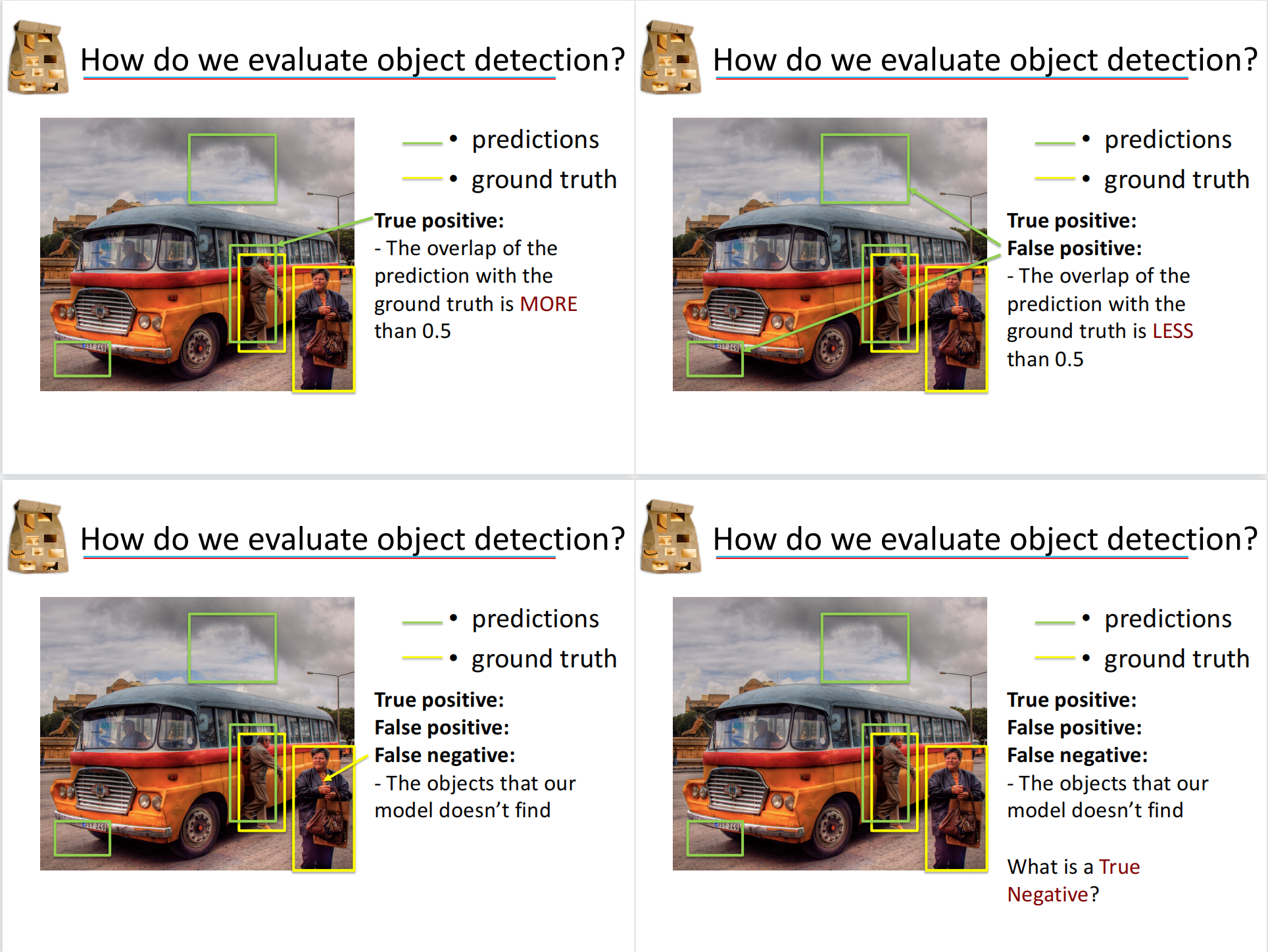
Four samples (TP, FP, FN, TN)
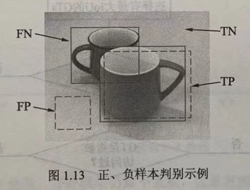
There are two cup labels in the diagram, and the model produces two prediction boxes.
Because there are background and object labels in the image, the prediction box is also divided into correct and error, so the following will occur during the evaluation 4 4 4 samples.
- Correct Check Box TP(True Positive): The prediction box matches the label box correctly, and the IoU between them is greater than 0.5 0.5 0.5, as shown in the lower right detection box.
- False Positive: Predicts the background as an object, such as the lower left detection box in the image, which usually has no more than the IoU of all the labels in the image 0.5 0.5 0.5 .
- FN(False Negative): The object that the model was supposed to detect was not detected by the model, such as the cup on the top left of the image.
- True Negative Background TN: It is the background itself, and the model is not detected, which is usually not considered in object detection.
Tips:
T/F: Model checked correctly
P/N: Is the model detected
Correct detection detected, target, TP; Detection error was detected again, using the background as an object, FP; Need to be detected but not detected, missed, FN; Detection is correct and does not require detection itself, background, TN.
With the above basics, we can begin to test the model.
Recall, Precision, mean Average Precision(mAP)
For a detector, mAP(mean Average Precision) is usually used to evaluate the quality of a model, where AP refers to the detection accuracy of one category and mAP is the average accuracy of multiple categories. Assessment requires the predicted and labeled values for each picture. For an example, they contain the following:
- Predicted value (Dets): the type of object, the position of the border 4 4 Four predictions, the score of the object.
- Tag value (GTs): Object class, border position 4 4 Four true values.
Based on the predicted and labeled values, the AP calculation process is shown in the figure. We first sort all the prediction boxes by score from high to low (because the higher the score, the more likely they are to be for real objects), and then traverse the prediction boxes from high to low.
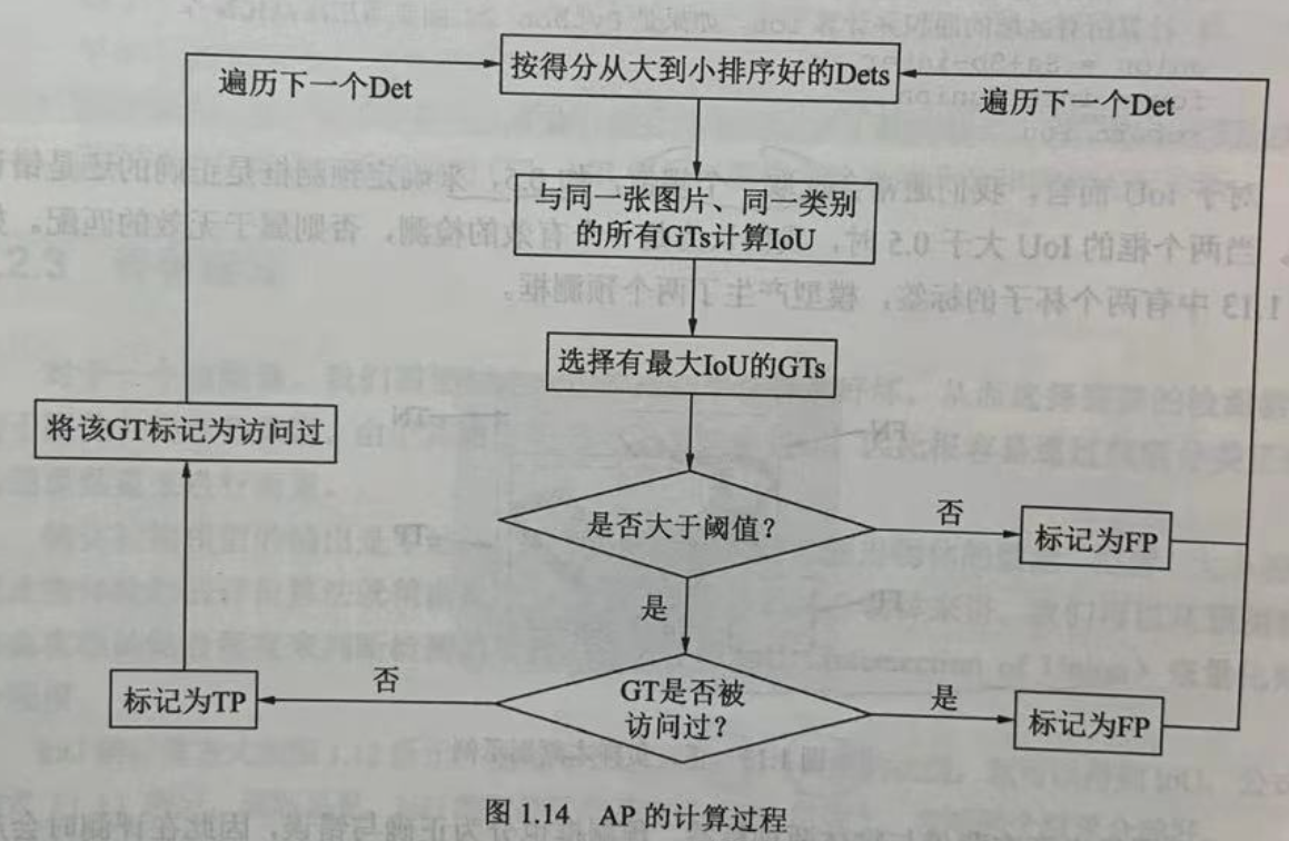
For a prediction box that is traversed, the IoU of all tag boxes GTs of the same category in the graph is calculated, and the GT with the largest IoU is selected as the matching object of the current prediction box. If the loU is less than the threshold, the current prediction box is marked as the false check box FP.
If the IoU is greater than the threshold, it also depends on whether the corresponding tag box GP has been accessed. If there is already a prediction box with a higher limit corresponding to the label box, it will be marked as FP even if the IoU is now larger than the threshold value. If not, mark the current prediction box Det as the correct check box TP and the GT as accessed to prevent subsequent prediction boxes from corresponding to it.
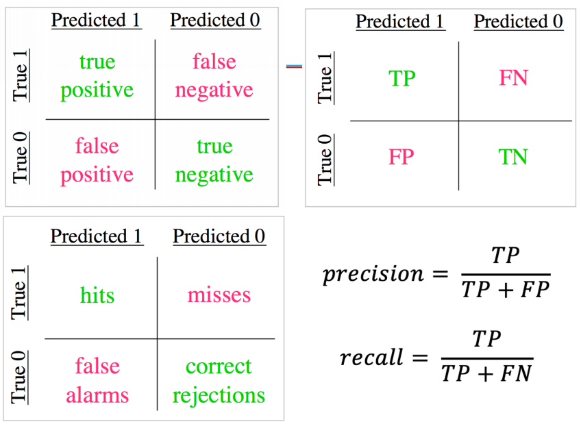
After traversing all the prediction boxes, we get the attributes of each prediction box, TP or FP. During traversal, we can calculate the model recall rate (Recall, R) by the current number of TP, that is, the ratio of the current total detected tag boxes to all tag boxes, as shown below. (Correct Detection/Correct Detection+Leak Detection)
R = T P l e n ( G T s ) = T P T P + F N R=\frac{TP}{len(GTs)}=\frac{TP}{TP+FN} R=len(GTs)TP=TP+FNTP
In addition to the recall rate, another important indicator is the accuracy (Precision, P), which is the ratio of the correctly predicted borders in the currently traversed prediction boxes, as shown below. (Correct Detection/Correct Detection+Error Detection)
P = T P T P + F P P=\frac{TP}{TP+FP} P=TP+FPTP
As you traverse each prediction box, you can generate a corresponding P and R, which can form a point ( R , P ) (R,P) (R,P), all points are plotted as curves, which form P-R curves, as shown in the figure.
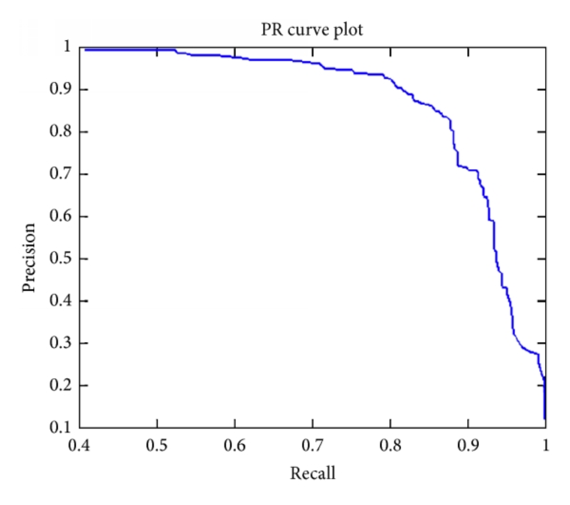
However, even with P-R curves, the evaluation model is still not intuitive. If the points on the curve are taken directly, it is not appropriate to select them anywhere, because the accuracy will be low when recall rate is high, and recall rate will be low when recall rate is high. At this point, AP comes in handy, and the calculation formula is shown in the formula.
A P = ∫ 0 1 P d R AP=\int_0^1P\mathrm{d}R AP=∫01PdR
As you can see from the formula, AP represents the area of the curve, taking into account the accuracy under different recall rates, and has no preference for P and R. The APs of each category are independent, and mAP can be obtained by averaging the APs of each category. Strictly speaking, the curve needs to be corrected before AP calculation. In addition to calculating area, you can also use 11 11 11 ways of averaging accuracy corresponding to different recall rates for AP.
Code implementation mAP
The following is a detailed code-level description of the AP solution process.
Folder data/detections is stored only 1 1 The detection information of one picture (n pictures of the real situation). Picture name is 1.jpg corresponding detection information is 1.txt.
Class,Left, Top, Right, Bottom, Score
File contents:
class1 12 58 53 96 0.87
class1 51 88 152 191 0.98
class2 345 898 431 945 0.67
class2 597 346 674 415 0.45
class1 243 546 298 583 0.83
class2 99 345 150 426 0.96
The folder data/groundtruths holds its true value information 1.txt.
Class, Left, Top, Right, Bottom
File contents:
class1 14 56 50 100
class1 50 90 150 189
class2 345 894 432 940
class1 458 657 580 742
class2 590 354 675 420
Assuming that both tag and prediction data are loaded, the following is required 3 3 Three variables:
- det_boxes: Contains the prediction boxes for all categories in all images, one of which contains [Ieft, top, right, bottom, score, NameofImage].
- gt_boxes: Contains labels for all categories in all images, one of which contains [left, top, right, bottom, 0]. Last 0 0 0 means whether the tag has been matched or not, if it has been matched it will be set to 1 1 1, the other prediction boxes are mismatched.
- num_pos: Includes the number of predictions for all categories in all images.
The following code generates two dictionary data types that meet the above image information requirements:
def getDetBoxes(DetFolder='./data/detections'):

    files = os.listdir(DetFolder)
    files.sort()

    det_boxes = {}
    for f in files:
        nameOfImage = f.replace(".txt", "")
        fh1 = open(os.path.join(DetFolder, f), "r")

        for line in fh1:
            line = line.replace("\n", "")
            if line.replace(' ', '') == '':
                continue
            splitLine = line.split(" ")

            # category
            cls = (splitLine[0])
            # coordinate
            left = float(splitLine[1])
            top = float(splitLine[2])
            right = float(splitLine[3])
            bottom = float(splitLine[4])
            # Confidence
            score = float(splitLine[5])
            # Name OfImage is the name of the picture, there is only one picture, name 1
            one_box = [left, top, right, bottom, score, nameOfImage]

            if cls not in det_boxes:
                det_boxes[cls]=[]
            det_boxes[cls].append(one_box)

        fh1.close()
    return det_boxes
def getGTBoxes(GTFolder='./data/groundtruths'):
    files = os.listdir(GTFolder)
    files.sort()

    classes = []
    num_pos = {}
    gt_boxes = {}
    for f in files:
        nameOfImage = f.replace(".txt", "")
        fh1 = open(os.path.join(GTFolder, f), "r")

        for line in fh1:
            line = line.replace("\n", "")
            if line.replace(' ', '') == '':
                continue
            splitLine = line.split(" ")

            # category
            cls = (splitLine[0])
            left = float(splitLine[1])
            # coordinate
            top = float(splitLine[2])
            right = float(splitLine[3])
            bottom = float(splitLine[4])
            # 0 means not visited
            one_box = [left, top, right, bottom, 0]

            # Category Name List
            if cls not in classes:
                classes.append(cls)
                gt_boxes[cls] = {}
                num_pos[cls] = 0

            num_pos[cls] += 1

            if nameOfImage not in gt_boxes[cls]:
                gt_boxes[cls][nameOfImage] = []
            gt_boxes[cls][nameOfImage].append(one_box)

        fh1.close()
    return gt_boxes, classes, num_pos
gt_boxes, classes_name, num_pos = getGTBoxes('./data/groundtruths')
det_boxes = getDetBoxes('./data/detections')
# ground truth
gt_boxes
{'class1': {'1': [[14.0, 56.0, 50.0, 100.0, 0],
   [50.0, 90.0, 150.0, 189.0, 0],
   [458.0, 657.0, 580.0, 742.0, 0]]},
 'class2': {'1': [[345.0, 894.0, 432.0, 940.0, 0],
   [590.0, 354.0, 675.0, 420.0, 0]]}}
# detection boxing
det_boxes
{'class1': [[12.0, 58.0, 53.0, 96.0, 0.87, '1'],
  [51.0, 88.0, 152.0, 191.0, 0.98, '1'],
  [243.0, 546.0, 298.0, 583.0, 0.83, '1']],
 'class2': [[345.0, 898.0, 431.0, 945.0, 0.67, '1'],
  [597.0, 346.0, 674.0, 415.0, 0.45, '1'],
  [99.0, 345.0, 150.0, 426.0, 0.96, '1']]}
classes_name
['class1', 'class2']
num_pos
{'class1': 3, 'class2': 2}
cfg = {'iouThreshold': 0.5} # configuration file

The IoU function is called following the above algorithm, and TP and FP are looped:
# AP calculation function
def AP_caculate(cfg, classes_name, det_boxes, gt_boxes, num_pos):
    # Configuration parameters, names of all categories, all prediction boxes, all label boxes, length of all prediction boxes
    ret = []
    for class_name in classes_name:
        # Using categories as keywords, get the predictions, labels, and total number of labels for each category
        dets = det_boxes[class_name]
        gt_class = gt_boxes[class_name]
        npos = num_pos[class_name]
        # Use score, the fourth element of dets, as the keyword to sort the prediction box by score
        dets = sorted(dets, key=lambda conf: conf[4], reverse=True)
        # Set two lists with the same length as the predicted border, marked as TP or FP
        TP = np.zeros(len(dets))
        FP = np.zeros(len(dets))
        # Traverse all prediction boxes for a category
        for d in range(len(dets)):
            # Minimize IoU by default
            IoUMax = sys.float_info.min
            # Calculate IoU by traversing labels of the same category in the same image as the prediction box
            if dets[d][-1] in gt_class:
                for j in range(len(gt_class[dets[d][-1]])):
                    iou = IoU(dets[d][: 4], gt_class[dets[d][-1]][j][:4])
                    if iou > IoUMax:
                        IoUMax = iou
                        jmax = j # Label with maximum IoU for record and forecast
                # If the maximum IoU is greater than the threshold and has not been matched, TP is assigned
                if IoUMax >= cfg['iouThreshold']:
                    if gt_class[dets[d][-1]][jmax][4] == 0:
                        TP[d] = 1
                        gt_class[dets[d][-1]][jmax][4] = 1 # Marked as matched
                    # If matched, assign FP
                    else:
                        FP[d] = 1
                # Assign FP if the maximum IoU does not exceed the threshold
                else:
                    FP[d] = 1
            # If there is no label for this category in the corresponding image, assign FP
            else:
                FP[d] = 1
        # Calculate cumulative FP and TP
        acc_FP = np.cumsum(FP)
        acc_TP = np.cumsum(TP)
        # Get Recall for each point, TP / len(GTs)
        rec = acc_TP / npos
        # Get Precision for each point, TP / TP + FP
        prec = np.divide(acc_TP, (acc_FP + acc_TP))
        # Calculate AP through Recall and recision
        [ap, m_pre, m_rec, ii] = CalculateAveragePrecision(rec, prec)
        r = {
                'class': class_name,
                'precision': prec,
                'recall': rec,
                'AP': ap,
                'interpolated precision': m_pre,
                'interpolated recall': m_rec,
                'total positives': npos,
                'total TP': np.sum(TP),
                'total FP': np.sum(FP),
            }
        ret.append(r)
    return ret, classes_name
After the Precision and Recall of each point are obtained, each discrete point is interpolated, and the AP is calculated by the discrete integral method:
# After getting P and R for each point, AP is calculated by discrete integral method
def CalculateAveragePrecision(rec, prec):
        m_rec = []
        m_rec.append(0)
        [m_rec.append(e) for e in rec] # List generation, add recall rate
        m_rec.append(1)

        m_pre = []
        m_pre.append(0)
        [m_pre.append(e) for e in prec] # List Generation, Add Precision
        m_pre.append(0)

        for i in range(len(m_pre) - 1, 0, -1):
            # Interpolation, greater precision between two points
            m_pre[i - 1] = max(m_pre[i - 1], m_pre[i])

        ii = []
        for i in range(len(m_rec) - 1):
            if m_rec[i + 1] != m_rec[i]:
                # Interpolation, taking recall s between two points only
                ii.append(i + 1)

        ap = 0
        for i in ii:
            # Discrete Integral
            ap = ap + np.sum((m_rec[i] - m_rec[i - 1]) * m_pre[i])

        return [ap, m_pre[0:len(m_pre) - 1], m_rec[0:len(m_pre) - 1], ii]
ret, class_name = AP_caculate(cfg, classes_name, det_boxes, gt_boxes, num_pos)
ret
[{'class': 'class1',
  'precision': array([1.        , 1.        , 0.66666667]),
  'recall': array([0.33333333, 0.66666667, 0.66666667]),
  'AP': 0.6666666666666666,
  'interpolated precision': [1.0, 1.0, 1.0, 0.6666666666666666],
  'interpolated recall': [0,
   0.3333333333333333,
   0.6666666666666666,
   0.6666666666666666],
  'total positives': 3,
  'total TP': 2.0,
  'total FP': 1.0},
 {'class': 'class2',
  'precision': array([0.        , 0.5       , 0.66666667]),
  'recall': array([0. , 0.5, 1. ]),
  'AP': 0.6666666666666666,
  'interpolated precision': [0.6666666666666666,
   0.6666666666666666,
   0.6666666666666666,
   0.6666666666666666],
  'interpolated recall': [0, 0.0, 0.5, 1.0],
  'total positives': 2,
  'total TP': 2.0,
  'total FP': 1.0}]
# AP for class1
ret[0]['AP']
0.6666666666666666
# Recall for each point after class 2 interpolation
ret[1]['interpolated recall']
[0, 0.0, 0.5, 1.0]
Target Detection Network Using Pre-training
The pre-training target detection networks of the R-CNN series are:
detection.fasterrcnn_resnet50_fpn
detection.maskrcnn_resnet50_fpn
detection.keypointrcnn_resnet50_fpn
# Model Load Selection GPU
device = torch.device("cuda" if torch.cuda.is_available() else "cpu")
print(device)
print(torch.cuda.device_count())
print(torch.cuda.get_device_name(0))
cuda
1
GeForce MX250
Image Target Detection
Use a pre-trained Fast R-CNN model with ResNet-50-FPN structure to train using COCO datasets
(COCO dataset download address: https://cocodataset.org)
# Import pre-trained ResNet50 Faster R-CNN model
model = torchvision.models.detection.fasterrcnn_resnet50_fpn(pretrained = True)
model = model.to(device)
model.eval()
FasterRCNN(
  (transform): GeneralizedRCNNTransform(
      Normalize(mean=[0.485, 0.456, 0.406], std=[0.229, 0.224, 0.225])
      Resize(min_size=(800,), max_size=1333, mode='bilinear')
  )
  (backbone): BackboneWithFPN(
    (body): IntermediateLayerGetter(
      (conv1): Conv2d(3, 64, kernel_size=(7, 7), stride=(2, 2), padding=(3, 3), bias=False)
      (bn1): FrozenBatchNorm2d(64, eps=0.0)
      (relu): ReLU(inplace=True)
      (maxpool): MaxPool2d(kernel_size=3, stride=2, padding=1, dilation=1, ceil_mode=False)
      (layer1): Sequential(
        (0): Bottleneck(
          (conv1): Conv2d(64, 64, kernel_size=(1, 1), stride=(1, 1), bias=False)
          (bn1): FrozenBatchNorm2d(64, eps=0.0)
          (conv2): Conv2d(64, 64, kernel_size=(3, 3), stride=(1, 1), padding=(1, 1), bias=False)
          (bn2): FrozenBatchNorm2d(64, eps=0.0)
          (conv3): Conv2d(64, 256, kernel_size=(1, 1), stride=(1, 1), bias=False)
          (bn3): FrozenBatchNorm2d(256, eps=0.0)
          (relu): ReLU(inplace=True)
          (downsample): Sequential(
            (0): Conv2d(64, 256, kernel_size=(1, 1), stride=(1, 1), bias=False)
            (1): FrozenBatchNorm2d(256, eps=0.0)
          )
        )
        (1): Bottleneck(
          (conv1): Conv2d(256, 64, kernel_size=(1, 1), stride=(1, 1), bias=False)
          (bn1): FrozenBatchNorm2d(64, eps=0.0)
          (conv2): Conv2d(64, 64, kernel_size=(3, 3), stride=(1, 1), padding=(1, 1), bias=False)
          (bn2): FrozenBatchNorm2d(64, eps=0.0)
          (conv3): Conv2d(64, 256, kernel_size=(1, 1), stride=(1, 1), bias=False)
          (bn3): FrozenBatchNorm2d(256, eps=0.0)
          (relu): ReLU(inplace=True)
        )
        (2): Bottleneck(
          (conv1): Conv2d(256, 64, kernel_size=(1, 1), stride=(1, 1), bias=False)
          (bn1): FrozenBatchNorm2d(64, eps=0.0)
          (conv2): Conv2d(64, 64, kernel_size=(3, 3), stride=(1, 1), padding=(1, 1), bias=False)
          (bn2): FrozenBatchNorm2d(64, eps=0.0)
          (conv3): Conv2d(64, 256, kernel_size=(1, 1), stride=(1, 1), bias=False)
          (bn3): FrozenBatchNorm2d(256, eps=0.0)
          (relu): ReLU(inplace=True)
        )
      )
      (layer2): Sequential(
        (0): Bottleneck(
          (conv1): Conv2d(256, 128, kernel_size=(1, 1), stride=(1, 1), bias=False)
          (bn1): FrozenBatchNorm2d(128, eps=0.0)
          (conv2): Conv2d(128, 128, kernel_size=(3, 3), stride=(2, 2), padding=(1, 1), bias=False)
          (bn2): FrozenBatchNorm2d(128, eps=0.0)
          (conv3): Conv2d(128, 512, kernel_size=(1, 1), stride=(1, 1), bias=False)
          (bn3): FrozenBatchNorm2d(512, eps=0.0)
          (relu): ReLU(inplace=True)
          (downsample): Sequential(
            (0): Conv2d(256, 512, kernel_size=(1, 1), stride=(2, 2), bias=False)
            (1): FrozenBatchNorm2d(512, eps=0.0)
          )
        )
        (1): Bottleneck(
          (conv1): Conv2d(512, 128, kernel_size=(1, 1), stride=(1, 1), bias=False)
          (bn1): FrozenBatchNorm2d(128, eps=0.0)
          (conv2): Conv2d(128, 128, kernel_size=(3, 3), stride=(1, 1), padding=(1, 1), bias=False)
          (bn2): FrozenBatchNorm2d(128, eps=0.0)
          (conv3): Conv2d(128, 512, kernel_size=(1, 1), stride=(1, 1), bias=False)
          (bn3): FrozenBatchNorm2d(512, eps=0.0)
          (relu): ReLU(inplace=True)
        )
        (2): Bottleneck(
          (conv1): Conv2d(512, 128, kernel_size=(1, 1), stride=(1, 1), bias=False)
          (bn1): FrozenBatchNorm2d(128, eps=0.0)
          (conv2): Conv2d(128, 128, kernel_size=(3, 3), stride=(1, 1), padding=(1, 1), bias=False)
          (bn2): FrozenBatchNorm2d(128, eps=0.0)
          (conv3): Conv2d(128, 512, kernel_size=(1, 1), stride=(1, 1), bias=False)
          (bn3): FrozenBatchNorm2d(512, eps=0.0)
          (relu): ReLU(inplace=True)
        )
        (3): Bottleneck(
          (conv1): Conv2d(512, 128, kernel_size=(1, 1), stride=(1, 1), bias=False)
          (bn1): FrozenBatchNorm2d(128, eps=0.0)
          (conv2): Conv2d(128, 128, kernel_size=(3, 3), stride=(1, 1), padding=(1, 1), bias=False)
          (bn2): FrozenBatchNorm2d(128, eps=0.0)
          (conv3): Conv2d(128, 512, kernel_size=(1, 1), stride=(1, 1), bias=False)
          (bn3): FrozenBatchNorm2d(512, eps=0.0)
          (relu): ReLU(inplace=True)
        )
      )
      (layer3): Sequential(
        (0): Bottleneck(
          (conv1): Conv2d(512, 256, kernel_size=(1, 1), stride=(1, 1), bias=False)
          (bn1): FrozenBatchNorm2d(256, eps=0.0)
          (conv2): Conv2d(256, 256, kernel_size=(3, 3), stride=(2, 2), padding=(1, 1), bias=False)
          (bn2): FrozenBatchNorm2d(256, eps=0.0)
          (conv3): Conv2d(256, 1024, kernel_size=(1, 1), stride=(1, 1), bias=False)
          (bn3): FrozenBatchNorm2d(1024, eps=0.0)
          (relu): ReLU(inplace=True)
          (downsample): Sequential(
            (0): Conv2d(512, 1024, kernel_size=(1, 1), stride=(2, 2), bias=False)
            (1): FrozenBatchNorm2d(1024, eps=0.0)
          )
        )
        (1): Bottleneck(
          (conv1): Conv2d(1024, 256, kernel_size=(1, 1), stride=(1, 1), bias=False)
          (bn1): FrozenBatchNorm2d(256, eps=0.0)
          (conv2): Conv2d(256, 256, kernel_size=(3, 3), stride=(1, 1), padding=(1, 1), bias=False)
          (bn2): FrozenBatchNorm2d(256, eps=0.0)
          (conv3): Conv2d(256, 1024, kernel_size=(1, 1), stride=(1, 1), bias=False)
          (bn3): FrozenBatchNorm2d(1024, eps=0.0)
          (relu): ReLU(inplace=True)
        )
        (2): Bottleneck(
          (conv1): Conv2d(1024, 256, kernel_size=(1, 1), stride=(1, 1), bias=False)
          (bn1): FrozenBatchNorm2d(256, eps=0.0)
          (conv2): Conv2d(256, 256, kernel_size=(3, 3), stride=(1, 1), padding=(1, 1), bias=False)
          (bn2): FrozenBatchNorm2d(256, eps=0.0)
          (conv3): Conv2d(256, 1024, kernel_size=(1, 1), stride=(1, 1), bias=False)
          (bn3): FrozenBatchNorm2d(1024, eps=0.0)
          (relu): ReLU(inplace=True)
        )
        (3): Bottleneck(
          (conv1): Conv2d(1024, 256, kernel_size=(1, 1), stride=(1, 1), bias=False)
          (bn1): FrozenBatchNorm2d(256, eps=0.0)
          (conv2): Conv2d(256, 256, kernel_size=(3, 3), stride=(1, 1), padding=(1, 1), bias=False)
          (bn2): FrozenBatchNorm2d(256, eps=0.0)
          (conv3): Conv2d(256, 1024, kernel_size=(1, 1), stride=(1, 1), bias=False)
          (bn3): FrozenBatchNorm2d(1024, eps=0.0)
          (relu): ReLU(inplace=True)
        )
        (4): Bottleneck(
          (conv1): Conv2d(1024, 256, kernel_size=(1, 1), stride=(1, 1), bias=False)
          (bn1): FrozenBatchNorm2d(256, eps=0.0)
          (conv2): Conv2d(256, 256, kernel_size=(3, 3), stride=(1, 1), padding=(1, 1), bias=False)
          (bn2): FrozenBatchNorm2d(256, eps=0.0)
          (conv3): Conv2d(256, 1024, kernel_size=(1, 1), stride=(1, 1), bias=False)
          (bn3): FrozenBatchNorm2d(1024, eps=0.0)
          (relu): ReLU(inplace=True)
        )
        (5): Bottleneck(
          (conv1): Conv2d(1024, 256, kernel_size=(1, 1), stride=(1, 1), bias=False)
          (bn1): FrozenBatchNorm2d(256, eps=0.0)
          (conv2): Conv2d(256, 256, kernel_size=(3, 3), stride=(1, 1), padding=(1, 1), bias=False)
          (bn2): FrozenBatchNorm2d(256, eps=0.0)
          (conv3): Conv2d(256, 1024, kernel_size=(1, 1), stride=(1, 1), bias=False)
          (bn3): FrozenBatchNorm2d(1024, eps=0.0)
          (relu): ReLU(inplace=True)
        )
      )
      (layer4): Sequential(
        (0): Bottleneck(
          (conv1): Conv2d(1024, 512, kernel_size=(1, 1), stride=(1, 1), bias=False)
          (bn1): FrozenBatchNorm2d(512, eps=0.0)
          (conv2): Conv2d(512, 512, kernel_size=(3, 3), stride=(2, 2), padding=(1, 1), bias=False)
          (bn2): FrozenBatchNorm2d(512, eps=0.0)
          (conv3): Conv2d(512, 2048, kernel_size=(1, 1), stride=(1, 1), bias=False)
          (bn3): FrozenBatchNorm2d(2048, eps=0.0)
          (relu): ReLU(inplace=True)
          (downsample): Sequential(
            (0): Conv2d(1024, 2048, kernel_size=(1, 1), stride=(2, 2), bias=False)
            (1): FrozenBatchNorm2d(2048, eps=0.0)
          )
        )
        (1): Bottleneck(
          (conv1): Conv2d(2048, 512, kernel_size=(1, 1), stride=(1, 1), bias=False)
          (bn1): FrozenBatchNorm2d(512, eps=0.0)
          (conv2): Conv2d(512, 512, kernel_size=(3, 3), stride=(1, 1), padding=(1, 1), bias=False)
          (bn2): FrozenBatchNorm2d(512, eps=0.0)
          (conv3): Conv2d(512, 2048, kernel_size=(1, 1), stride=(1, 1), bias=False)
          (bn3): FrozenBatchNorm2d(2048, eps=0.0)
          (relu): ReLU(inplace=True)
        )
        (2): Bottleneck(
          (conv1): Conv2d(2048, 512, kernel_size=(1, 1), stride=(1, 1), bias=False)
          (bn1): FrozenBatchNorm2d(512, eps=0.0)
          (conv2): Conv2d(512, 512, kernel_size=(3, 3), stride=(1, 1), padding=(1, 1), bias=False)
          (bn2): FrozenBatchNorm2d(512, eps=0.0)
          (conv3): Conv2d(512, 2048, kernel_size=(1, 1), stride=(1, 1), bias=False)
          (bn3): FrozenBatchNorm2d(2048, eps=0.0)
          (relu): ReLU(inplace=True)
        )
      )
    )
    (fpn): FeaturePyramidNetwork(
      (inner_blocks): ModuleList(
        (0): Conv2d(256, 256, kernel_size=(1, 1), stride=(1, 1))
        (1): Conv2d(512, 256, kernel_size=(1, 1), stride=(1, 1))
        (2): Conv2d(1024, 256, kernel_size=(1, 1), stride=(1, 1))
        (3): Conv2d(2048, 256, kernel_size=(1, 1), stride=(1, 1))
      )
      (layer_blocks): ModuleList(
        (0): Conv2d(256, 256, kernel_size=(3, 3), stride=(1, 1), padding=(1, 1))
        (1): Conv2d(256, 256, kernel_size=(3, 3), stride=(1, 1), padding=(1, 1))
        (2): Conv2d(256, 256, kernel_size=(3, 3), stride=(1, 1), padding=(1, 1))
        (3): Conv2d(256, 256, kernel_size=(3, 3), stride=(1, 1), padding=(1, 1))
      )
      (extra_blocks): LastLevelMaxPool()
    )
  )
  (rpn): RegionProposalNetwork(
    (anchor_generator): AnchorGenerator()
    (head): RPNHead(
      (conv): Conv2d(256, 256, kernel_size=(3, 3), stride=(1, 1), padding=(1, 1))
      (cls_logits): Conv2d(256, 3, kernel_size=(1, 1), stride=(1, 1))
      (bbox_pred): Conv2d(256, 12, kernel_size=(1, 1), stride=(1, 1))
    )
  )
  (roi_heads): RoIHeads(
    (box_roi_pool): MultiScaleRoIAlign(featmap_names=['0', '1', '2', '3'], output_size=(7, 7), sampling_ratio=2)
    (box_head): TwoMLPHead(
      (fc6): Linear(in_features=12544, out_features=1024, bias=True)
      (fc7): Linear(in_features=1024, out_features=1024, bias=True)
    )
    (box_predictor): FastRCNNPredictor(
      (cls_score): Linear(in_features=1024, out_features=91, bias=True)
      (bbox_pred): Linear(in_features=1024, out_features=364, bias=True)
    )
  )
)
# Preparing images for detection
image = Image.open('./data/objdetect/2012_004308.jpg')
transform_d = transforms.Compose([transforms.ToTensor()])
image_t = transform_d(image).to(device) # Image transformation
pred = model([image_t]) # Output Prediction
pred
[{'boxes': tensor([[139.8201,  35.2344, 306.0309, 211.2748],
          [ 78.5456, 117.7256, 294.9999, 274.1726],
          [176.4146,  45.9989, 293.7729, 167.6908],
          [446.5353, 298.2009, 482.5389, 332.6683],
          [144.3929,  59.9620, 242.3081, 232.6723],
          [264.5503, 289.4034, 348.2632, 330.4233],
          [ 81.9035,  99.5320, 306.7264, 279.0831],
          [304.1234,  68.3819, 500.0000, 314.6510],
          [246.3921,  79.3525, 495.8307, 323.0642],
          [264.6102, 288.0742, 348.0310, 330.5592]], device='cuda:0',
         grad_fn=<StackBackward>),
  'labels': tensor([ 1,  2,  1,  1,  1, 15,  4,  5,  2,  8], device='cuda:0'),
  'scores': tensor([0.9954, 0.9430, 0.8601, 0.8108, 0.4989, 0.3326, 0.3135, 0.1794, 0.1665,
          0.1197], device='cuda:0', grad_fn=<IndexBackward>)}]
Boxes are bounding boxes.
labels are the categories to which the target belongs.
Scores are scores belonging to the corresponding category (i.e. confidence objectness).
Detection Content Visualization
Define labels for each category:
COCO_INSTANCE_CATEGORY_NAMES = [
    '__background__', 'person', 'bicycle', 'car', 'motorcycle',
    'airplane', 'bus', 'train', 'truck', 'boat', 'traffic light',
    'fire hydrant', 'N/A', 'stop sign', 'parking meter', 'bench',
    'bird', 'cat', 'dog', 'horse', 'sheep', 'cow', 'elephant',
    'bear', 'zebra', 'giraffe', 'N/A', 'backpack', 'umbrella', 'N/A',
    'N/A', 'handbag', 'tie', 'suitcase', 'frisbee', 'skis', 'snowboard',
    'sports ball', 'kite', 'baseball bat', 'baseball glove', 'skateboard',
    'surfboard', 'tennis racket', 'bottle', 'N/A', 'wine glass',
    'cup', 'fork', 'knife', 'spoon', 'bowl', 'banana', 'apple',
    'sandwich', 'orange', 'broccoli', 'carrot', 'hot dog', 'pizza',
    'donut', 'cake', 'chair', 'couch', 'potted plant', 'bed', 'N/A',
    'dining table', 'N/A', 'N/A', 'toilet', 'N/A', 'tv', 'laptop',
    'mouse', 'remote', 'keyboard', 'cell phone', 'microwave', 'oven',
    'toaster', 'sink', 'refrigerator', 'N/A', 'book', 'clock',
    'vase', 'scissors', 'teddy bear', 'hair drier', 'toothbrush'
]
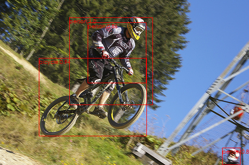
Before visualization, you need to interpret the valid prediction target data separately, extracting information about each target's location, category, and score, and then scoring more than 0 , 5 0,5 Targets of 0,5 are detected as valid targets, and the detected targets are displayed on the image.
# Detected target categories and scores
pred_class = [COCO_INSTANCE_CATEGORY_NAMES[ii] for ii in list(pred[0]['labels'].cpu().numpy())]
pred_score = list(pred[0]['scores'].detach().cpu().numpy())
# Detecting the bounding box of the target
pred_boxes = [[ii[0], ii[1], ii[2], ii[3]] for ii in list(pred[0]['boxes'].detach().cpu().numpy())]
# Keep only those with recognition probability greater than 0.5
pred_index = [pred_score.index(x) for x in pred_score if x > 0.5]
# Set font for image display
fontsize = np.int16(image.size[1] / 30)
font1 = ImageFont.truetype('C:/windows/Fonts/STXIHEI.TTF', fontsize) # Chinese Fine Black
# Visualize Images
draw = ImageDraw.Draw(image)
for index in pred_index:
    box = pred_boxes[index]
    draw.rectangle(box, outline = 'red')
    texts = pred_class[index] + ':' + str(np.round(pred_score[index], 2))
    draw.text((box[0], box[1]), texts, fill = 'red', font = font1)
image
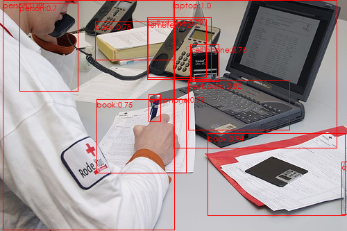
The target detection process described above is defined as a function to facilitate the detection of any image:
def Object_Detect(model, image_path, COCO_INSTANCE_CATEGORY_NAMES, threshold = 0.5):
    image = Image.open(image_path)
    transform_d = transforms.Compose([transforms.ToTensor()])
    image_t = transform_d(image).to(device) # Image transformation
    pred = model([image_t]) # Output Prediction
    # Detect target categories and scores
    pred_class = [COCO_INSTANCE_CATEGORY_NAMES[ii] for ii in list(pred[0]['labels'].cpu().numpy())]
    pred_score = list(pred[0]['scores'].detach().cpu().numpy())
    # Detecting the bounding box of the target
    pred_boxes = [[ii[0], ii[1], ii[2], ii[3]] for ii in list(pred[0]['boxes'].detach().cpu().numpy())]
    # Keep only results where recognition probability is greater than threshold
    pred_index = [pred_score.index(x) for x in pred_score if x > threshold]
    # Set font for image display
    fontsize = np.int16(image.size[1] / 30)
    font1 = ImageFont.truetype('C:/windows/Fonts/STXIHEI.TTF', fontsize) # Chinese Fine Black
    # Visual images and detection results
    draw = ImageDraw.Draw(image)
    for index in pred_index:
        box = pred_boxes[index]
        draw.rectangle(box, outline = 'red')
        texts = pred_class[index] + ':' + str(np.round(pred_score[index], 2))
        draw.text((box[0], box[1]), texts, fill = 'red', font = font1)
    return image
# Call the above function
image_path = './data/objdetect/2012_003924.jpg'
Object_Detect(model, image_path, COCO_INSTANCE_CATEGORY_NAMES, 0.7)