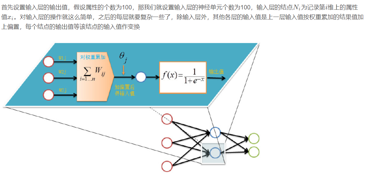
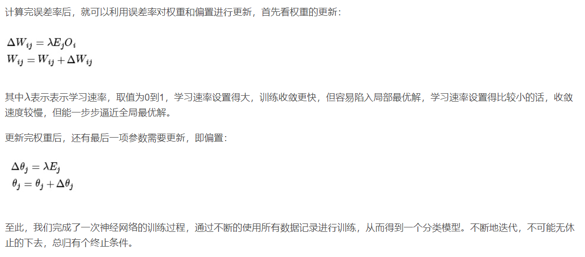
1, Introduction

1 Overview
BP (Back Propagation) neural network was proposed by the scientific research group headed by Rumelhart and McCelland in 1986. See their paper learning representations by Back Propagation errors published in Nature.

BP neural network is a multilayer feedforward network trained by error back propagation algorithm. It is one of the most widely used neural network models at present. BP network can learn and store a large number of input-output mode mapping relationships without revealing the mathematical equations describing this mapping relationship in advance. Its learning rule is to use the steepest descent method and continuously adjust the weight and threshold of the network through back propagation to minimize the sum of squares of the network error.

2 basic idea of BP algorithm
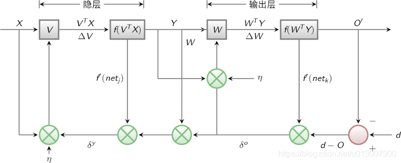
Last time, we said that multilayer perceptron encountered a bottleneck in how to obtain the weight of hidden layer. Since we can't get the weight of the hidden layer directly, can we indirectly adjust the weight of the hidden layer by getting the error between the output result and the expected output from the output layer first? BP algorithm is designed with this idea. Its basic idea is that the learning process consists of two processes: forward propagation of signal and back propagation of error.
During forward propagation, the input samples are transmitted from the input layer, processed layer by layer by hidden layer, and then transmitted to the output layer. If the actual output of the output layer is inconsistent with the expected output (teacher signal), it will turn to the back propagation stage of error.
During back propagation, the output is transmitted back to the input layer layer by layer through the hidden layer in some form, and the error is allocated to all units of each layer, so as to obtain the error signal of each layer unit, which is used as the basis for correcting the weight of each unit.
The specific processes of these two processes will be introduced later.

The signal flow diagram of BP algorithm is shown in the figure below

3 characteristic analysis of BP network -- three elements of BP
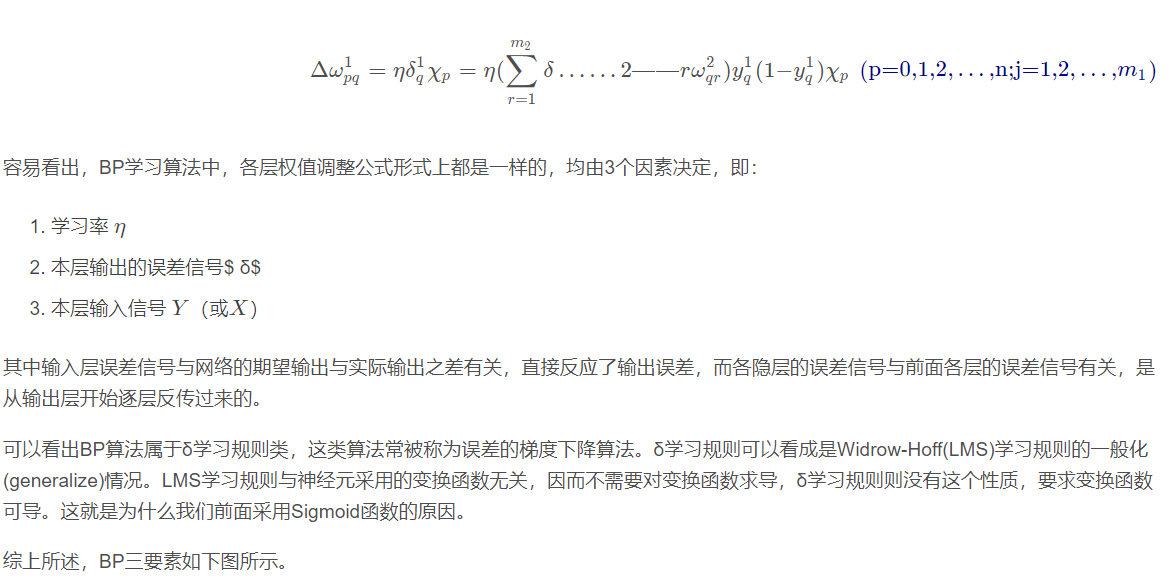
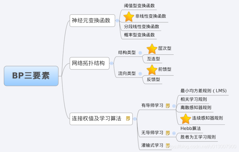
When we analyze an ANN, we usually start with its three elements, namely
1) Network topology;
2) Transfer function;
3) Learning algorithm.

The characteristics of each element together determine the functional characteristics of the ANN. Therefore, we also study BP network from these three elements.
3.1 topology of BP network
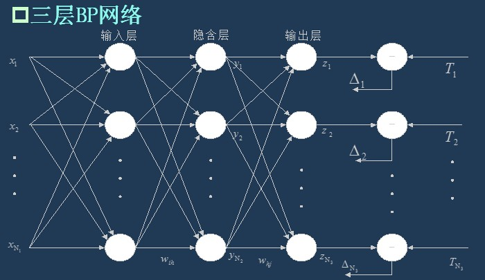
As I said last time, BP network is actually a multilayer perceptron, so its topology is the same as that of multilayer perceptron. Because the single hidden layer (three-layer) perceptron can solve simple nonlinear problems, it is most widely used. The topology of the three-layer perceptron is shown in the figure below.
The simplest three-tier BP:

3.2 transfer function of BP network
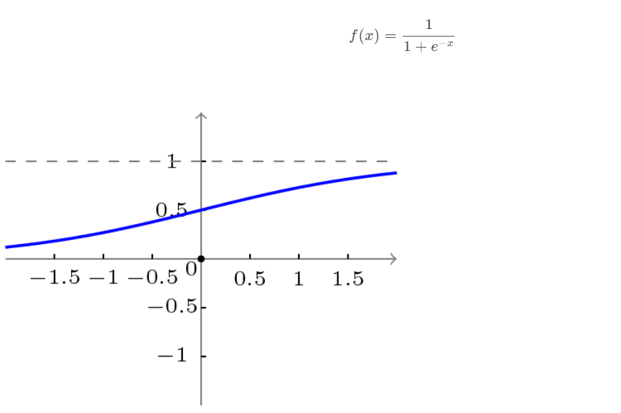
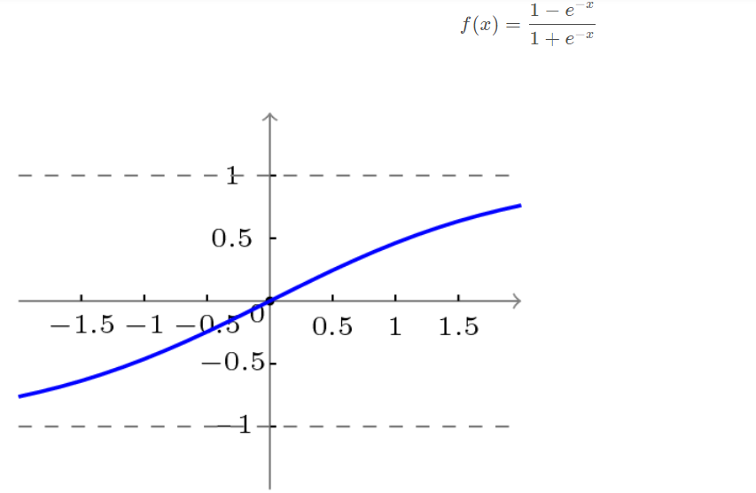
The transfer function adopted by BP network is a nonlinear transformation function - Sigmoid function (also known as S function). Its characteristic is that the function itself and its derivatives are continuous, so it is very convenient in processing. Why should we choose this function? I will give a further introduction when introducing the learning algorithm of BP network.
Unipolar S-type function curve is shown in the figure below.

The bipolar S-type function curve is shown in the figure below.

3.3 learning algorithm of BP network
The learning algorithm of BP network is BP algorithm, also known as BP algorithm δ Algorithm (in the learning process of ANN, we will find many terms with multiple names). Taking the three-layer perceptron as an example, when the network output is different from the expected output, there is an output error E, which is defined as follows




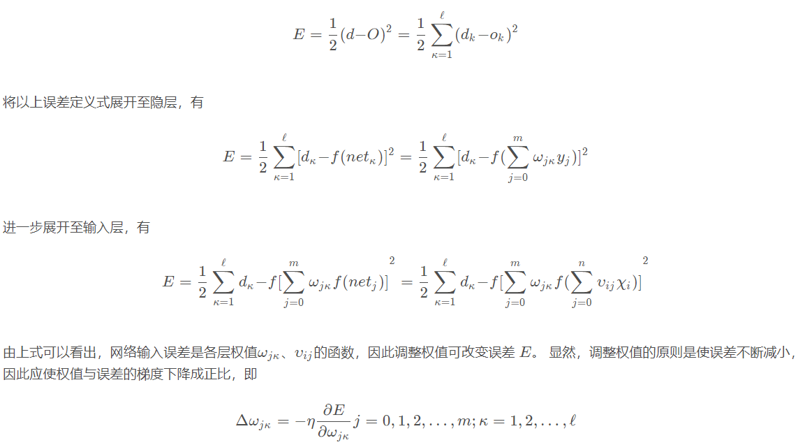
Next, we will introduce the specific process of BP network learning and training.

4 training decomposition of BP network
Training a BP neural network is actually adjusting the weight and bias of the network. The training process of BP neural network is divided into two parts:

Forward transmission, wave transmission output value layer by layer;
Reverse feedback, reverse layer by layer adjustment of weight and bias;
Let's first look at forward transmission.
Forward transmission (feed forward feedback)
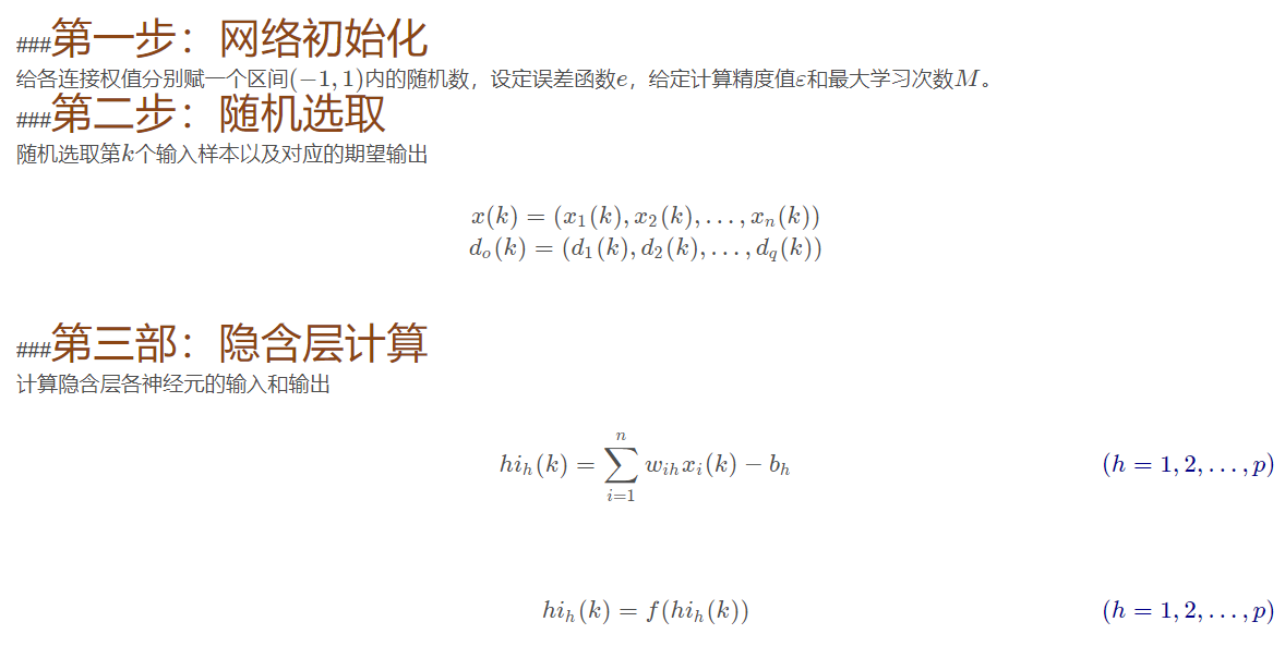
Before training the network, we need to initialize weights and offsets randomly, take a random real number of [− 1,1] [- 1,1] [− 1,1] for each weight, and a random real number of [0,1] [0,1] [0,1] for each offset, and then start forward transmission.

The training of neural network is completed by multiple iterations. Each iteration uses all records of the training set, while each training network uses only one record. The abstract description is as follows:

while Termination conditions not met:
    for record:dataset:
        trainModel(record)

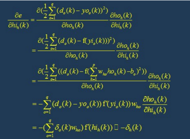
4.1 back propagation


4.2 training termination conditions
Each round of training uses all records of the data set, but when to stop, there are two stopping conditions:
Set the maximum number of iterations, such as stopping training after 100 iterations with the dataset
Calculate the prediction accuracy of the training set on the network, and stop the training after reaching a certain threshold

5. Specific process of BP network operation
5.1 network structure
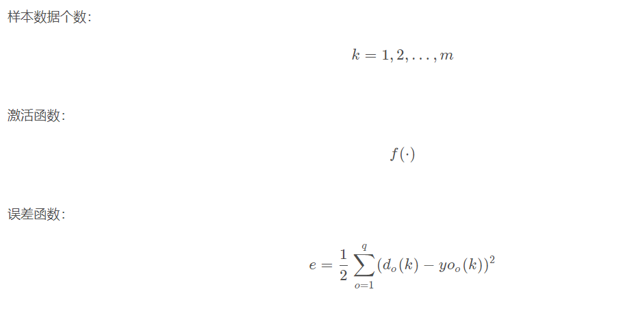
There are n nn neurons in the input layer, p pp neurons in the hidden layer and q qq neurons in the output layer.
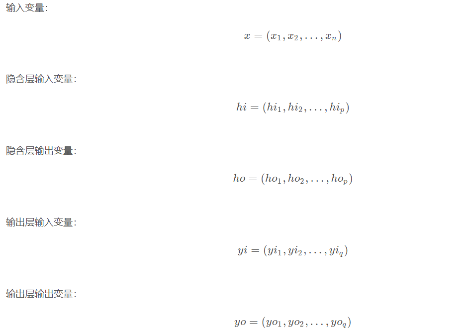
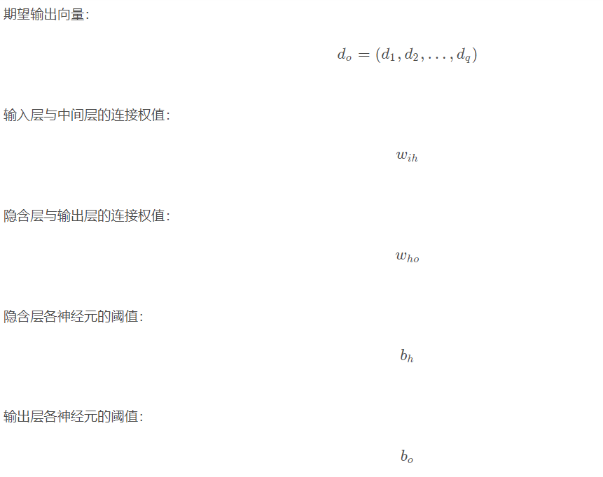
5.2 variable definition








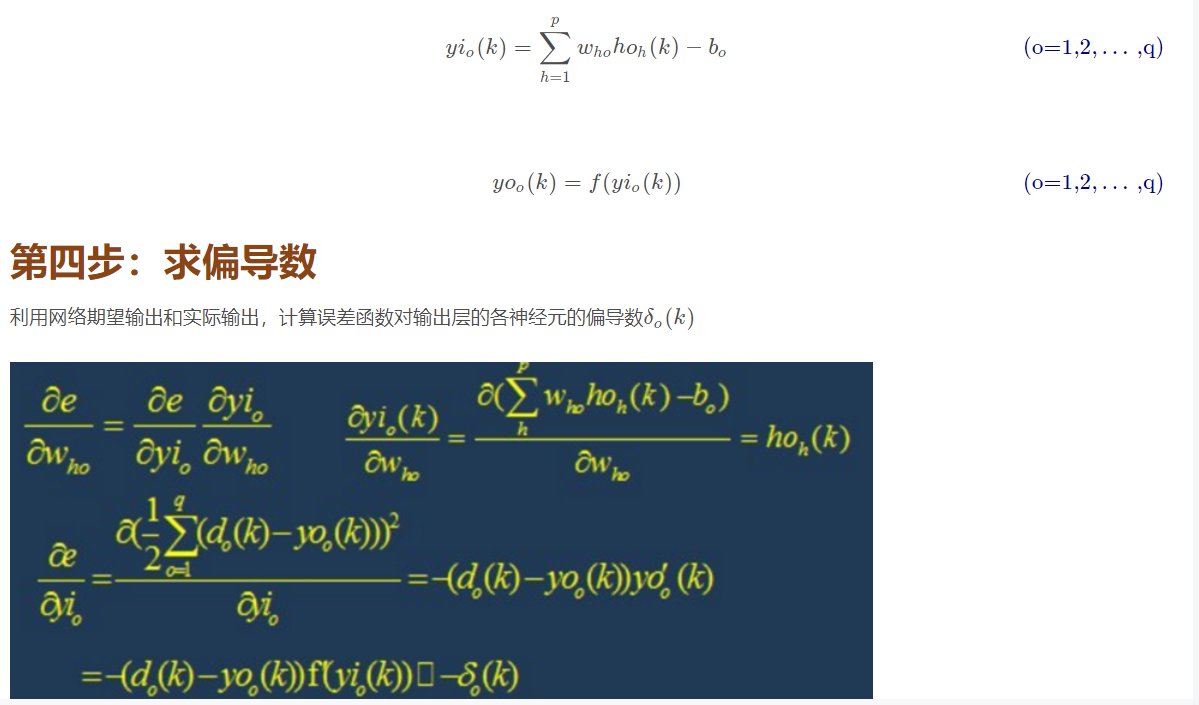
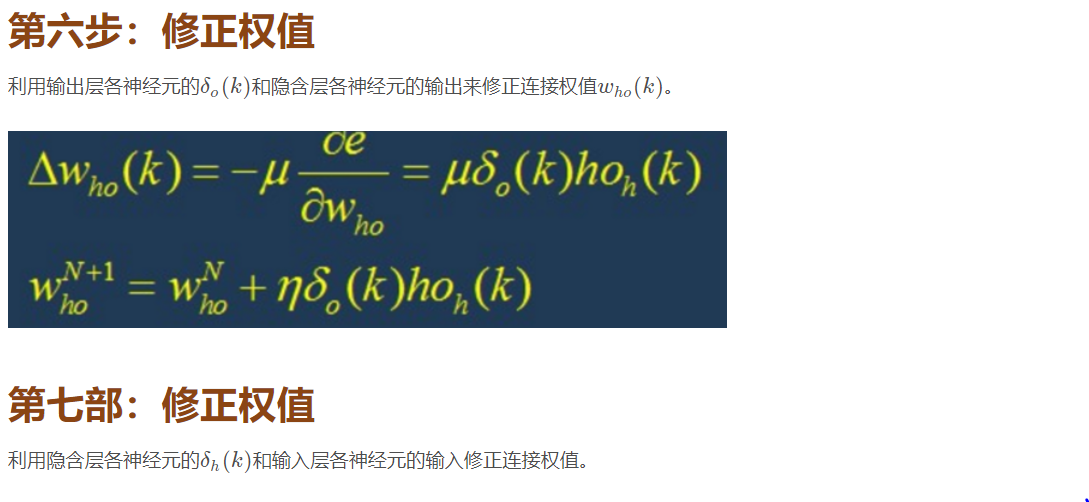
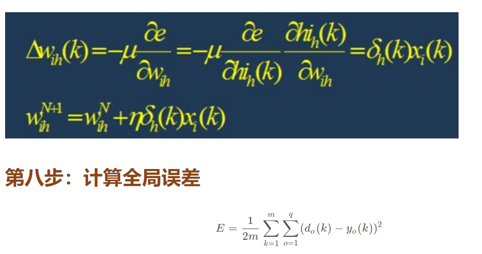
Step 9: judge the rationality of the model
Judge whether the network error meets the requirements.
When the error reaches the preset accuracy or the learning times are greater than the designed maximum times, the algorithm is ended.
Otherwise, select the next learning sample and the corresponding output expectation, return to the third part and enter the next round of learning.

6 design of BP network
In the design of BP network, we should generally consider the number of layers of the network, the number of neurons and activation function in each layer, initial value and learning rate. The following are some selection principles.
6.1 layers of network
Theory has proved that the network with deviation and at least one S-type hidden layer plus a linear output layer can approach any rational function. Increasing the number of layers can further reduce the error and improve the accuracy, but it is also the complexity of the network. In addition, the single-layer network with only nonlinear activation function can not be used to solve the problem, because the problem that can be solved with single-layer network can also be solved with adaptive linear network, and the operation speed of adaptive linear network is faster. For the problem that can only be solved with nonlinear function, the single-layer accuracy is not high enough, and only increasing the number of layers can achieve the desired result.
6.2 number of neurons in the hidden layer
The improvement of network training accuracy can be obtained by using a hidden layer and increasing the number of neurons, which is much simpler in structure than increasing the number of network layers. Generally speaking, we use the accuracy and the time of training the network to measure the quality of a neural network design:
(1) When the number of neurons is too small, the network can not learn well, the number of training iterations is relatively large, and the training accuracy is not high.
(2) When there are too many neurons, the more powerful the function of the network is, the higher the accuracy is, and the number of training iterations is also large, which may lead to over fitting.
Therefore, we get the selection principle of the number of neurons in the hidden layer of neural network: on the premise of solving the problem, add one or two neurons to speed up the decline of error.

6.3 selection of initial weight
Generally, the initial weight is a random number with a value between (− 1,1). In addition, after analyzing how the two-layer network trains a function, wedrow et al. Proposed a strategy to select the initial weight order as s √ r, where r is the number of inputs and S is the number of neurons in the first layer.

6.4 learning rate
The learning rate is generally 0.01 − 0.8. A large learning rate may lead to the instability of the system, but a small learning rate leads to too slow convergence and requires a long training time. For more complex networks, different learning rates may be required at different positions of the error surface. In order to reduce the training times and time to find the learning rate, a more appropriate method is to use the variable adaptive learning rate to set different learning rates in different stages.

6.5 selection of expected error
In the process of designing the network, the expected error value should also determine an appropriate value after comparative training, which is determined relative to the required number of hidden layer nodes. In general, two networks with different expected error values can be trained at the same time, and finally one of them can be determined by comprehensive factors.

7 limitations of BP network
BP network has the following problems:

(1) It needs a long training time: This is mainly caused by the small learning rate, which can be improved by changing or adaptive learning rate.
(2) Completely unable to train: This is mainly reflected in the paralysis of the network. Generally, in order to avoid this situation, one is to select a smaller initial weight, but use a smaller learning rate.
(3) Local minimum value: the gradient descent method adopted here may converge to the local minimum value, and it is possible to obtain better results by using multi-layer network or more neurons.

8 improvement of BP network
The main goal of the improvement of P algorithm is to speed up the training speed and avoid falling into local minima. The common improvement methods include the algorithm with momentum factor, adaptive learning rate, changing learning rate and action function contraction method. The basic idea of momentum factor method is to add a value proportional to the previous weight change to each weight change on the basis of back propagation, and generate a new weight change according to the back propagation method. The method of adaptive learning rate is aimed at some specific problems. The principle of the method of changing the learning rate is that if the sign of the objective function for the reciprocal of a weight is the same in several consecutive iterations, the learning rate of this weight will increase, on the contrary, if the sign is opposite, the learning rate will decrease. The contraction rule of the action function is to translate the action function, that is, add a constant.

2, Source code

clear all;
%Form user interface and add graphic window
H=figure('Color',[0.75 0.75 0.75],...
    'position',[400 200 500 400],...
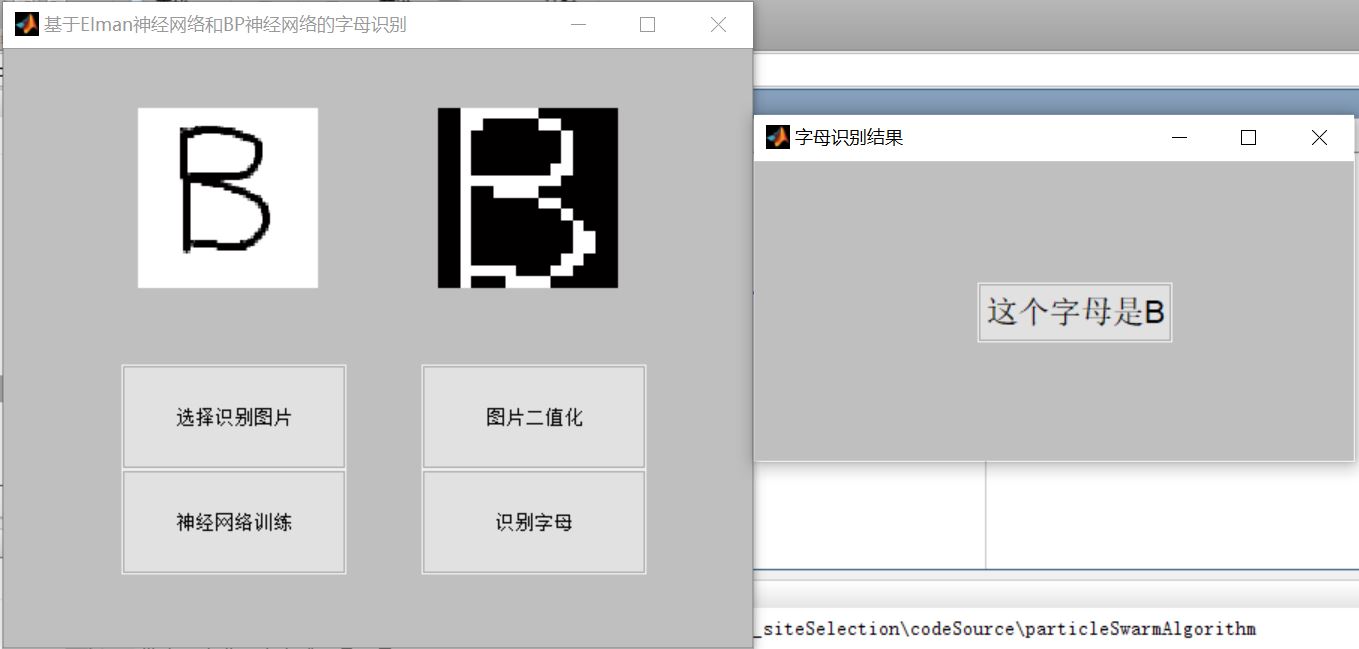
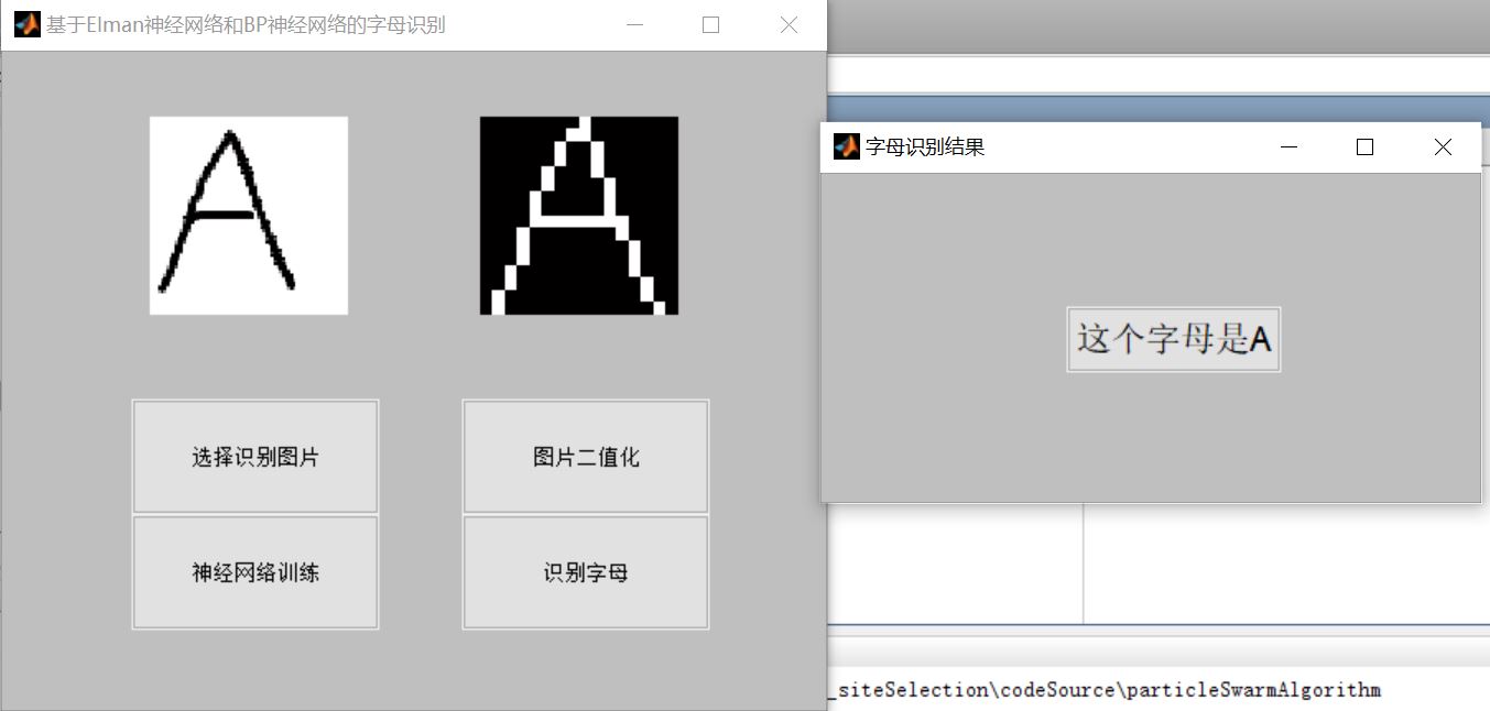
    'Name','be based on Elman Neural networks and BP Letter recognition based on Neural Network',...
    'NumberTitle','off',...
    'MenuBar','none');
%Draw the coordinate axis object and display the original image
h0=axes('position',[0.15 0.6 0.3 0.3]);
%Add image open button
h1=uicontrol(H,'Style','push',...
    'Position',[80 120 150 70],...
    'String','Select recognition picture',...
    'FontSize',10,...
    'Call','op');
%Draw the coordinate axis object and display the preprocessed image
h2=axes('position',[0.55 0.6 0.3 0.3]);
%Add preprocessing button
h3=uicontrol(H,'Style','push',...
    'Position',[280 120 150 70],...
    'String','Image binarization',...
    'FontSize',10,...
    'Call','preprocess');
%Add recognition button
h4=uicontrol(H,'Style','push',...
    'Position',[280 50 150 70],...
    'String','Identifying letters',...
    'FontSize',10,...
    'Call','recognize');
%Add a text box that displays the recognition results
%recognize
%Generating vector form
M=figure('Color',[0.75 0.75 0.75],...
    'position',[200 300 400 200],...
    'Name','Letter recognition results',...
    'NumberTitle','off',...
    'MenuBar','none');
M0=uicontrol(M,'Style','push',...
    'Position',[150 80 130 40],...
    'String','Please train the network first',...
    'FontSize',12,...
       'call','delete(M(1)) ' );  

for m=0:15
    q(m*16+1:(m+1)*16,1)=p1(1:16,m+1);
end
%Identification display
[a,Pf,Af]=sim(net,q);
a=round(a);
switch a
    case 0,M0=uicontrol(M,'Style','push',...
    'Position',[150 80 130 40],...
    'String','This letter is A',...
    'FontSize',16,...
    'call',...
    'delete(M(1))'); 
    case 1,M0=uicontrol(M,'Style','push',...
    'Position',[150 80 130 40],...
    'String','This letter is B',...
    'FontSize',16,...
    'call',...
    'delete(M(1))'); 
    case 2,M0=uicontrol(M,'Style','push',...
    'Position',[150 80 130 40],...
    'String','This letter is C',...
    'FontSize',16,...
    'call',...
    'delete(M(1))'); 
    case 3,M0=uicontrol(M,'Style','push',...
    'Position',[150 80 130 40],...
    'String','This letter is D',...
    'FontSize',16,...
    'call',...
    'delete(M(1))'); 
    case 4,M0=uicontrol(M,'Style','push',...
    'Position',[150 80 130 40],...
    'String','This letter is E',...
    'FontSize',16,...
    'call',...
    'delete(M(1))'); 
    case 5,M0=uicontrol(M,'Style','push',...
    'Position',[150 80 130 40],...
    'String','This letter is F',...
    'FontSize',16,...
    'call',...
    'delete(M(1))'); 
    case 6,M0=uicontrol(M,'Style','push',...
    'Position',[150 80 130 40],...
    'String','This letter is G',...
    'FontSize',16,...
    'call',...
    'delete(M(1))'); 
    case 7,M0=uicontrol(M,'Style','push',...
    'Position',[150 80 130 40],...
    'String','This letter is H',...
    'FontSize',16,...
    'call',...
    'delete(M(1))'); 
    case 8,M0=uicontrol(M,'Style','push',...
    'Position',[150 80 130 40],...
    'String','This letter is I',...
    'FontSize',16,...
    'call',...
    'delete(M(1))'); 
    case 9,M0=uicontrol(M,'Style','push',...
    'Position',[150 80 130 40],...
    'String','This letter is J',...
    'FontSize',16,...
    'call',...
    'delete(M(1))'); 
    case 10,M0=uicontrol(M,'Style','push',...
    'Position',[150 80 130 40],...
    'String','This letter is K',...
    'FontSize',16,...
    'call',...
    'delete(M(1))'); 
    case 11,M0=uicontrol(M,'Style','push',...
    'Position',[150 80 130 40],...
    'String','This letter is L',...
    'FontSize',16,...
    'call',...
    'delete(M(1))'); 

3, Operation results

4, Remarks

Complete code or write on behalf of QQ 1564658423