Multi objective genetic algorithm
In this paper, the optimization model of non optimal supplier is established by considering the idea of Pareto 2. In addition, the optimization model of non optimal supplier and non optimal supplier is transformed into multiple objective solutions. In addition, the genetic algorithm is used to minimize the cost of each supplier. In this paper, the optimization problem of non optimal supplier and non optimal supplier is solved at the same time, That is, the obtained schemes have advantages in two optimization objectives. Algorithm steps:
Step1: enter the problem data and the relevant parameters of functional service providers, including the number n of suppliers, unit transportation cost, unit value-added service cost, fixed fee, transportation distance, maximum business commitment, as well as the expected quality and perceived quality of service supply.
Step 2: set algorithm parameters, population size N and maximum number of iterations Max_gen, crossover probability Pc, mutation probability Pm, iteration counter k=1.
Step 3: population initialization. The solution code of the logistics service provider selection problem is a set of permutations represented by 0-1
, if supplier i is selected to provide logistics services
, otherwise
; N groups of permutations are randomly generated to form the initial population, but it needs to be verified that the random solution meets the two constraints of the minimum number of suppliers and the maximum business commitment is not less than the demand. If the above two constraints are not met, the random solution needs to be regenerated.
Step4: calculate the target value of the initial population. ① decoding operation. According to the objective function of the lower level planning, only the suppliers with high customer service satisfaction index can ensure the maximum global customer satisfaction; Therefore, when allocating the freight volume of suppliers, the suppliers with high customer service satisfaction index shall provide goods in turn to achieve their maximum business commitment as far as possible. Some selected suppliers in the initial solution may not be allocated to the business volume, so it is necessary to modify the initial solution to make the supplier i allocated the business volume in the initial solution
. ② Calculate the cost of suppliers according to formula (1) and the modified initial solution, and calculate the customer satisfaction index according to formula (2) and the business volume of each supplier after decoding operation.
Step5: crossover operation: pair the population individuals randomly and generate a random probability that obeys the uniform distribution of (0, 1). If the random probability is less than the crossover probability Pc, the crossover operation will be carried out, otherwise it will not be carried out. Specific contents of crossover operation: randomly generate two intersections, exchange the elements of two paired individuals between the intersections, generate two new solutions, judge whether the new solution meets the two constraints of the minimum number of suppliers and the maximum business commitment is not less than the demand. If it is true, keep the new solution to the crossover population, otherwise discard the new solution.
Step6: mutation operation: generate n random probabilities obeying (0, 1) uniform distribution for each supplier, judge whether the random probability is less than the mutation probability Pm, and if so, change the supplier's
The value of is replaced by alleles, and the new solution is retained to the mutant population.
Step 7: merge the target population and the crossover population, and calculate the initial value of the target population.
Step 8: screen the non inferior solutions, calculate the dominant relationship of the non inferior solutions in the combined population, and determine the non inferior solution set Q.
Step9: update the population and count the number of non inferior solutions in the non inferior solution set Q. if it is less than the population size N, multiple random initial solutions will be randomly generated to supplement to maintain the scale of the new initial population. Otherwise, N non inferior solutions will be randomly selected to form a new initial population.
Step10: algorithm termination condition, judge K < Max_ Gen, if true, make k=k+1 and go to step 5.
Step11: output the optimal solution, output the non inferior solution set Q, decode the non inferior solution, and obtain the modified non inferior solution, the business volume of each supplier and the corresponding two target values.
explain
1. dominate and non inferior in multi-standard optimization problems, if at least one goal of individual p is better than that of individual Q, and all goals of individual p are not worse than that of individual Q, then individual p dominates individual Q (p dominates q), or individual q is dominated by individual p (q is dominated by p), Individual p is not inferior to individual Q (p Is non- inferior to g).
2. rank and f ront end
If P dominates q, then the order value of P is lower than that of q. If P and q do not dominate each other, or if P and q are not inferior to each other, then p and q have the same order value. Individuals with an order value of 1 belong to the first front end, individuals with an order value of 2 belong to the second front end, and so on. Obviously, in the current population, the first front end is completely uncontrolled, and the second front end is dominated by the individuals in the first front end. In this way, individuals in the population can be divided into different front ends through sorting.
3. crowding distance
Crowding distance is used to calculate the distance between an individual in a front end and other individuals in the front end to characterize the crowding degree between individuals. Obviously, the larger the crowding distance, the less crowding among individuals and the better the diversity of the population. It should be pointed out that only individuals in the same front end need to calculate the congestion distance, and it is meaningless for individuals in different front ends to calculate the congestion distance.
code
clc;clear;
tic;
%% initialization
PopSize=200;%Population size
MaxIteration =200;%Maximum number of iterations
R=50;
load('cc101');
shuju=c101;
bl=0;
cap=800; %Maximum vehicle load
%% Extract data information
E=shuju(1,5); %Start time of distribution center time window
L=shuju(1,6); %End time of distribution center time window
zuobiao=shuju(:,2:3); %Coordinates of all points x and y
% vertexs= vertexs./1000;
customer=zuobiao(2:end,:); %Customer coordinates
cusnum=size(customer,1); %Number of customers
v_num=6; %Maximum number of vehicles used
demands=shuju(2:end,4); %requirement
a=shuju(2:end,5); %Customer time window start time[a[i],b[i]]
b=shuju(2:end,6); %End time of customer time window[a[i],b[i]]
s=shuju(2:end,7); %Customer service time
h=pdist(zuobiao);
% dist=load('dist1.mat');
% dist=struct2cell(dist);
% dist=cell2mat(dist);
% dist=dist./1000; %Distance between actual cities
location1=squareform(h); %The distance matrix satisfies the triangular relationship and temporarily uses the distance to represent the cost c[i][j]=dist[i][j]
%% Genetic algorithm parameter setting
alpha=100000; %Penalty function coefficients for violating capacity constraints
belta=900;%Penalty function coefficient for violation of time window constraint
belta2=60;
chesu=0.667;
N=cusnum+v_num-1; %Chromosome length=Number of customers+Maximum number of vehicles used-1
% location1=load('location1_100.txt');%Optimize 100 cities
% location2=load('A_location2_100.txt');
% location1=load('location1.txt');
% location2=load('location2.txt');
% CityNum =size(location1,2);%Number of cities
V=N;
M=2;
pc=0.8;pm=0.9;
%% Initialize population
init_vc=init(cusnum,a,demands,cap); %Construct initial solution
chromosome(:,1:N)=InitPopCW(PopSize,N,cusnum,init_vc);
% for i=1:PopSize
% % chromosome(i,1:CityNum)=randperm(CityNum);
% chromosome(i,V+1:V+2)=costfunction(chromosome(i,1:V),location1,location2);
% end
chromosome(:,V+1:V+2)=calObj(chromosome,cusnum,cap,demands,a,b,L,s,location1,alpha,belta,belta2,chesu,bl); %Calculate the value of population objective function
%%
[chromosome,individual]= non_domination_sort_mod(chromosome,N);%The last column of the solution is the last to last of the congestion degree, and the second column is the classification number
index=find(chromosome(:,N+3)==1);
costrep=chromosome(index,N+1:N+2);%First order non inferior solution
%% Main cycle
pool = round(PopSize/2); %Mutation pool scale
for Iteration=1:MaxIteration
if ~mod(Iteration,10)
fprintf('current iter:%d\n',Iteration)
disp([' Number of Repository Particles = ' num2str(size(costrep,1))]);
end
parent_chromosome = selection_individuals(chromosome,pool,2);
parent_var=parent_chromosome(:,1:N);%Separate the solution vector
%% overlapping
offspring_var=[];offspring_cost=[];
for ic=1:pool/2
m1=randi(pool);%Select the cross vector
m2=randi(pool);
while m1==m2
m1=randi(pool);
end
scro(1,:)=parent_var(m1,:);
scro(2,:)=parent_var(m2,:);
if rand<pc
c1=randi(N);%Select the crossing position
c2=randi(N);
while c1==c2
c1=randi(N);
end
chb1=min(c1,c2);
chb2=max(c1,c2);
middle=scro(1,chb1+1:chb2);
scro(1,chb1+1:chb2)=scro(2,chb1+1:chb2);
scro(2,chb1+1:chb2)=middle;
for i=1:chb1
while find(scro(1,chb1+1:chb2)==scro(1,i))
zhi=find(scro(1,chb1+1:chb2)==scro(1,i));
y=scro(2,chb1+zhi);
scro(1,i)=y;
end
while find(scro(2,chb1+1:chb2)==scro(2,i))
zhi=find(scro(2,chb1+1:chb2)==scro(2,i));
y=scro(1,chb1+zhi);
scro(2,i)=y;
end
end
for i=chb2+1:N
while find(scro(1,1:chb2)==scro(1,i))
zhi=find(scro(1,1:chb2)==scro(1,i));
y=scro(2,zhi);
scro(1,i)=y;
end
while find(scro(2,1:chb2)==scro(2,i))
zhi=find(scro(2,1:chb2)==scro(2,i));
y=scro(1,zhi);
scro(2,i)=y;
end
end
end
if rand<pm%Reverse order variation
m1=randi(N);
m2=randi(N);
while m1==m2
m1=randi(N);
end
loc1=min(m1,m2);loc2=max(m1,m2);
scro(1,loc1:loc2)=fliplr(scro(1,loc1:loc2));
% tt=scro(1,m2);
% scro(1,m2)=scro(1,m1);
% scro(1,m1)=tt;
end
if rand<pm%Reciprocal variation
m1=randi(N);
m2=randi(N);
while m1==m2
m1=randi(N);
end
tt=scro(2,m2);
scro(2,m2)=scro(2,m1);
scro(2,m1)=tt;
end
scro_cost(1,:)=calObj(scro(1,:),cusnum,cap,demands,a,b,L,s,location1,alpha,belta,belta2,chesu,bl);
% scro_cost(1,:)=costfunction(scro(1,:),location1,location2);
scro_cost(2,:)=calObj(scro(2,:),cusnum,cap,demands,a,b,L,s,location1,alpha,belta,belta2,chesu,bl);
% scro_cost(2,:)=costfunction(scro(2,:),location1,location2);
offspring_var=[offspring_var;scro];%solution
offspring_cost=[offspring_cost;scro_cost];%Fitness
end
offspring_chromosome(:,1:V)=offspring_var;
offspring_chromosome(:,V+1:V+M)=offspring_cost;
main_pop = size(chromosome,1);
offspring_pop = size(offspring_chromosome,1);
intermediate_chromosome(1:main_pop,:) = chromosome;
intermediate_chromosome(main_pop + 1 :main_pop + offspring_pop,1 : M+V) = ...
offspring_chromosome;
intermediate_chromosome = ...
non_domination_sort_mod(intermediate_chromosome,N);
%% choice
chromosome = replace_chromosome(intermediate_chromosome,PopSize,N);
index=find(intermediate_chromosome(:,N+3)==1);
costrep=intermediate_chromosome(index,N+1:N+2);
cost=intermediate_chromosome(:,N+1:N+2);
if ~mod(Iteration,1)
figure (1)
plot(costrep(:,1),costrep(:,2),'r*',cost(:,1),cost(:,2),'kx');
xlabel('F1');ylabel('F2');
title(strcat('Interaction ',num2str(Iteration), ' Pareto non-dominated solutions'));
% hold on
end
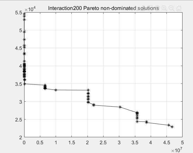
if ~mod(Iteration,MaxIteration)
% if ~mod(Iteration,1)
fun_pf=costrep;
[fun_pf,~]=sortrows(fun_pf,1);
plot(fun_pf(:,1),fun_pf(:,2),'k*-');
title(strcat('Interaction ',num2str(Iteration), ' Pareto non-dominated solutions'));
hold on;
grid on;
end
end
result
According to your own understanding, you can choose the appropriate one first, and the two functions are distance and time penalty cost.
If you have any questions, contact: VX: zzs1056600403