• 📢 Blog home page: https://blog.csdn.net/weixin_43197380
• 📢 Welcome to like 👍 Collection ⭐ Leaving a message. 📝 Please correct any mistakes!
• 📢 This article was originally written by Loewen and was first published in CSDN and reprinted with the source indicated 🙉
• 📢 Now pay, will be a kind of precipitation, just to make you a better person ✨

preface

Defect detection algorithm is different from size, QR code, OCR and other algorithms. The application scenario of the latter is relatively simple and basically applies some mature operators, so the threshold is low and it is easier to make standardized tools. The defect detection has the characteristics of the industry, and the defect algorithms of different industries are quite different. The common thing is to detect the surface defects of articles, such as spots, pits, scratches, color differences, defects and other defects on the workpiece surface. With the improvement of defect detection requirements, machine learning and deep learning have become an indispensable technical difficulty in the defect field. Next, I will make a simple analysis of standard defect detection algorithms and non-standard algorithms in the semiconductor industry:

1. Defect detection classification

1.1 standard defect detection

The so-called standards are not aimed at the characteristics of the industry. They are basically divided into the following categories:

• Standard preprocessing functions: image enhancement, corrosion, expansion, open operation, close operation, filtering, Fourier transform (frequency domain spatial domain conversion), distance transform, difference, etc
• Area detection: calculate the area within ROI after threshold
• Blob (threshold segmentation + feature extraction) detection: calculate blob after threshold connection
• Concentration difference detection: calculate the maximum concentration, minimum concentration and concentration difference within the ROI range
• Burr / defect on straight line / curve: fit the straight line / curve and calculate the distance from the edge point to the straight line / curve

The standard approach is generally to combine standard algorithm blocks to achieve the effect of defect detection. The standard process of defect detection is generally as follows:

1 set reference map template - > 2 locate current map template - > 3 generate affine transformation matrix - > 4 rotate and translate image or region - > 5 preprocess difference - > 6 preprocess filtering / corrosion / expansion - > 7 blob detection - > 8 area detection

1.2 non standard defect detection (for industry characteristics)

Compared with standard practices, there are many non-standard practices. Some non-standard practices are designed to reduce operation steps, such as turning the above combined process into a tool, which we call business logic non-standard. There are also some non-standard image preprocessing parts, such as modifying some standard preprocessing operators and preprocessing processes to extract defects. Of course, friends who have a good grasp of mathematical theory will deduce theoretical formulas, and then directly realize the mathematical formulas to achieve the detection effect.

2. Industry difficulties

• Traditional algorithms detect defects: it is difficult to debug, it is easy to adjust parameters repeatedly in the case of unstable detection, and there are many complex defects, false detection and poor compatibility
• Machine learning defect detection: generally, some single-layer neural networks similar to MLP are used to train and classify the defect features. This method needs to extract the defect part in advance, which is generally used in combination with the traditional segmentation method to achieve the effect of defect detection and classification.
• Deep learning defect detection (labeling): generally, customers need to provide a large number of defect samples, and the more types of defects and the less obvious characteristics, the larger defect samples are needed. Secondly, the labeling process is difficult to be automatic. It needs manual assistance to frame the defect location, and the workload is very large. The conclusion is that the training cycle is long and the training samples are large. If the customer can provide a large number of samples, this method is the first choice (the semiconductor industry generally does not have a large number of defective samples)
• Deep learning defect detection (transfer learning method): I think this method will become a general trend of defect detection in later industrial fields, but some companies need to collect defect type pictures and training network models of various industries and share them (suddenly it feels like a business opportunity, it depends on who can seize it), Then we can use the method of transfer learning to learn the model trained by others.

3. Conventional defect detection algorithm (Halcon)

In general, defect detection algorithms include:

• Blob analysis + feature extraction (commonly used, relatively simple)
• Positioning (Blob positioning, template matching positioning) + differential (common)
• Photometric stereo
• Characteristic training
• Measurement fitting (common)
• Frequency domain + spatial domain combination (common)
• Deep learning

3.1 difference method

I think there are a lot of standard defect detection methods. As the name suggests, difference is to find out the different regions by making a difference between two images or two regions. The processing flow is basically the way of positioning Blob analysis + difference or template matching + difference, which is mainly used to detect the damage, bulge, hole, loss, quality detection, etc. The specific processes of the two methods are as follows:

3.1.1 blob analysis + difference

The detection process is as follows:

1. Read image
2. Blob analysis is performed on the image to extract the Roi detection area on the image
3. Perform differential processing directly on the Roi area or with the image without defects
   ps: here, the difference includes area difference and image difference.
4. Finally, find the difference set, and judge whether the article is defective according to the area of the difference set
   Algorithm analysis: take the gray value in the standard image as the template, calculate the gray value of the detection image at the position, and make a difference with the standard image. The greater the gray value difference, it is proved that there is an area with obvious gray change compared with the standard image in the detection image, that is, this part of the area is the defect area we want to screen out.

Example analysis: extract the defect area with obvious gray value

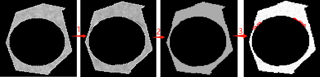
*1.use`intensity()`The operator calculates the average gray value of the detection area image of the template image (i.e. standard image, Fig. 1)`OriginalMean`
intensity(OriginalRegion, ImageReduced1, OriginalMean, Deviation1) 
 
*2.again`intensity()`The operator calculates the average gray value of the detection area image of the image to be measured (Fig. 2)`DetectMean`，Calculate the difference between the gray mean of the two images
intensity (DetectRegion, ImageReduced2, DetectMean, Deviation2)
tuple_abs (OriginalMean-DetectMean, Abs)
 
*3.
*If the gray value difference between the two areas is greater than 10( if(Abs>10))，Then an image is generated (Fig. 3), and its gray value is the average gray value calculated in the template image;  
*If the gray value difference between the two areas is less than 10( if(Abs<10))，Then an image is generated (Fig. 3), and its gray value is the average gray value calculated in the map to be measured.
*ps: The calculation result here is that the difference is less than 10, that is, there is little difference between the gray value of the detection image and the template image, and a gray mean image of the latter is directly generated
if(Abs>10)
   gen_image_proto (ImageReduced2, ImageCleared, OriginalMean)
else
   gen_image_proto (ImageReduced2, ImageCleared, DetectMean)
endif
reduce_domain (ImageCleared, RegionDifference, ImageReduced1)
 
*4.By making the difference between the image to be measured and the newly generated gray value image (Fig. 4), we can find the area where the gray value of the image to be measured is different from that of the template image
abs_diff_image (ImageReduced2, ImageReduced1, ImageAbsDiff, 1)
invert_image (ImageAbsDiff, ImageInvert)
threshold (ImageInvert, Region1, 0, 30)
opening_circle (Region1, RegionOpening, 1.5)
connection (RegionOpening, ConnectedRegions)
select_shape (ConnectedRegions, SelectedRegions, 'area', 'and', 10, 99999)

The test results are as follows:

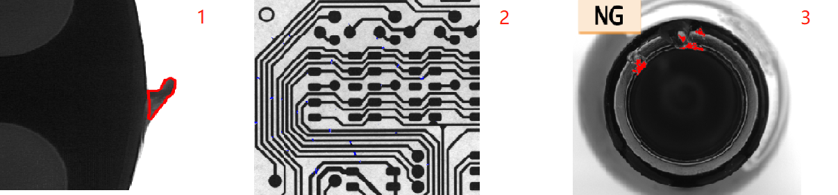
If you don't understand, list some differential routines in Halcon:

1. Detect burrs( Blob + difference method)- fin.hdev

2. Circuit board defect detection (Blob + difference method) - pcb_inspection.hdev

3. Bottle mouth damage defect detection (Blob + difference method) - inspect_bottle_mouth.hdev (pay attention to the conversion between rectangular coordinate system and polar coordinate system)

3.1.2 template matching + difference

The process is as follows:

1. First locate the template area, obtain the coordinates of the template area, and create the shape template of the article_ shape_ Model, pay attention to change the rotation angle of the template to rad(0) and rad(360)
2. Match template find_ shape_ During model, the shape is partially changed due to the defect of the article, so set MinScore smaller, otherwise it will not match the template. And get the coordinates of the matching items
3. The key step is to affine transform the template region to the region with successful matching. Because the difference operation works in the same region, the template region must be converted to the matching region
4. Finally, find the difference set, and judge whether the article is defective according to the area of the difference set

Example analysis: printing quality defect detection( Realizable template matching + difference method)- print_check.hdev

ps: there is no difference in it, but the special difference operator provided by Halcon for the deformation template: compare_variation_model();

3.1.3 comparison of two detection methods

Blob analysis is applicable to the situation that the whole image needs to be Roi region or Roi region somewhere in the image can be easily extracted through preprocessing. When blob analysis cannot locate the R region of the image, template matching is needed. Locate the Roi region of the image through template matching (shape matching or local deformation matching), and then use the difference model to detect defects. It can be understood that template matching + difference is an advanced version of blob analysis + difference, which can be easily handled and can be handed over to son blob analysis, If it's difficult, Dad can match the template.

3.2 frequency domain + space combination method

3.2.1 Fourier transform theory

Fourier transform is a transformation of function in space domain and frequency domain. The transformation from space domain to frequency domain is Fourier transform, while the transformation from frequency domain to space domain is the inverse of Fourier transform.

Time domain and frequency domain:

• Frequency domain
  It refers to analyzing the part related to frequency rather than time when analyzing a function or signal. It is opposite to the word time domain.
• Time domain (spatial domain)
  It describes the relationship between mathematical function or physical signal and time. For example, the time domain waveform of a signal can express the change of the signal over time. If discrete time is considered, the value of the function or signal in the time domain at each discrete time point is known. If continuous time is considered, the value of function or signal at any time is known. When studying the signal in time domain, oscilloscope is often used to convert the signal into its time domain waveform.
• Transformation between the two
  The transformation of time domain (signal to time function) and frequency domain (signal to frequency function) is mathematically realized by integral transformation. Fourier transform can be directly used for periodic signals, and Laplace transform should be used for periodic expansion of aperiodic signals.

Signal performance in frequency domain:

In the frequency domain, the higher the frequency, the faster the change speed of the original signal; The brighter the frequency, the smoother the original signal. When the frequency is 0, it indicates that the DC signal does not change. Therefore, the frequency reflects the speed of signal change. The high-frequency component explains the abrupt part of the signal, while the low-frequency component determines the overall image of the signal.

In image processing, frequency reflects the intensity of image gray change in spatial domain, that is, the change speed of image gray, that is, the gradient of image. In the frequency domain, the change of the edge component is fast, so it is the change of the edge component of the image in the frequency domain; In most cases, the noise of the image is the high-frequency part; The gently changing part of the image is a low-frequency component. In other words, Fourier transform provides another angle to observe the image, which can transform the image from gray distribution to frequency distribution to observe the characteristics of the image. To put it in writing, Fourier transform provides a way of free conversion from airspace to frequency. For image processing, the following concepts are very important.

By Cloth cloth The "first image cup boxing challenge championship" with full title officially begins. Please:

• High frequency team contestants: noise, detail and edge
  Image high frequency component: image mutation part, in some cases, refers to image edge information, in some cases, refers to noise, and it is more a mixture of the two.
• Low frequency team contestants: overall image outline
  Image low-frequency component: the part of the image (brightness / gray) that changes gently, which represents an area with continuous gradient. This part is low-frequency. For an image, the one that removes the high frequency is the low frequency, that is, the content within the edge is the low frequency, and the content within the edge is most of the information of the image, that is, the general outline and outline of the image, which is the approximate information of the image.
• Pro high frequency referee representative: high pass filter - let the high-frequency component of the image pass through and suppress the low-frequency component.
• Pro low frequency referee representative: low pass filter - contrary to high pass, let the low-frequency component of the image pass through and suppress the high-frequency component.
• Representative of the iron face: bandpass filter - enables the frequency information of an image in a certain part to pass through, and suppresses other too low or too high.
• Representative of the referee: band stop filter is the inverse of band-pass.

Enhance understanding: image noise is generally white or black spots, because it is different from the normal point color, that is, the gray value of the pixel is obviously different, that is, the gray changes rapidly, so it is the high-frequency part; The details of the image also belong to the area where the gray value changes rapidly. It is precisely because of the sharp change of the gray value that the details appear, which also belongs to the high-frequency part; Therefore, generally, the signal will be processed by low-pass filtering first, that is, the high-frequency part (noise / detail / edge) in the image will be filtered out, leaving the low-frequency (image contour), and the result is that the image is blurred.

ps: in image processing, some books say low-frequency response contour and high-frequency response details; Some articles say that the low-frequency response is the background, and the high-frequency response is the edge; Low frequency response contour. Here, the contour does not refer to the edge (many people will be confused and think that the contour refers to the edge). For example, when a nearsighted person takes off his glasses, people usually say, "I can't see anything clearly, but can only see a general contour." It means something similar. Therefore, the edge extraction of the image is still the high-frequency information of the edge. These two statements are not contradictory.

Summary: low frequency represents the overall image contour, high frequency represents image noise, edge and detail, and medium frequency represents image texture.

3.2.2 application scenarios

Application scenarios for frequency domain analysis using Fourier transform:

1. For images with certain texture features, the texture can be understood as stripes, such as cloth, wood, paper and other materials are easy to appear.
2. It is necessary to extract features with low contrast or low signal-to-noise ratio.
3. The image size is large or needs to be calculated with a large-size filter. At this time, it is converted to frequency domain calculation, which has the advantage of speed. Because the spatial domain filtering is a convolution process (weighted summation), the frequency domain calculation is multiplied directly.

3.2.3 core detection operator

In Halcon, the idea of using the frequency domain for detection is to filter appropriately in the frequency domain from the spatial domain to the frequency domain, select the desired frequency band, and then return to the spatial domain. There are two key steps:

1. Generate appropriate filter

Corresponding key operators:

gen_std_bandpass
gen_sin_bandpass
*Create a Gaussian filter, sigma The smaller the filter is, the smaller the signal passing through is more concentrated in the low frequency. The purpose of this is to get the background
gen_gauss_filter( : ImageGauss : Sigma1, Sigma2, Phi, Norm, Mode, Width, Height : )((common)
gen_mean_filter
gen_derivative_filter
gen_bandpass
gen_bandfilter
gen_highpass
gen_lowpass

2. Fast Fourier transform (mutual conversion between spatial domain and frequency domain)

Corresponding key operators:

fft_generic(Image : ImageFFT : Direction, Exponent, Norm, Mode, ResultType : )
rft_generic(Image : ImageFFT : Direction, Norm, ResultType, Width : )

The two operators have in common:

These two operators can transform the spatial domain - > frequency domain and the frequency domain - > spatial domain. They only need to select the parameter Direction separately, and the parameter 'to'_ Freq 'is the transformation from spatial domain to frequency domain,' from_freq 'is the transformation from frequency domain to space domain

For the parameter ResultType, if it is to_freq ', then the ResultType generally selects' complex'; If 'from'_ Freq ', ResultType generally selects' byte' (grayscale image).

The two operators are different:

fft_generic: the position of the DC item in the frequency domain can be in the upper left corner (Mode: 'dc_edge') or the origin can be shifted to the center (Mode: 'dc_center')

rft_generic: the item Mode is not set, and the origin is in the upper left corner by default.

In addition, fft_image: it can also perform fast Fourier transform (from spatial domain to frequency domain), which is equivalent to fft_generic(Image,ImageFFT,‘to_freq’,-1,‘sqrt’,‘dc_center’,‘complex’)

3.2.4 relevant actual test cases

🐨 Defect detection on the surface of plastic products_ indent_ fft. hdev

* 1.For pictures of the specified size fft Speed optimization
optimize_rft_speed (Width, Height, 'standard')
Sigma1 := 10.0
Sigma2 := 3.0
* 2.Construct two Gaussian filters, ps: Sigma The selection of parameters is very important
gen_gauss_filter (GaussFilter1, Sigma1, Sigma1, 0.0, 'none', 'rft', Width, Height)
gen_gauss_filter (GaussFilter2, Sigma2, Sigma2, 0.0, 'none', 'rft', Width, Height)
* Subtraction of two pictures (grayscale)
sub_image (GaussFilter1, GaussFilter2, Filter, 1.025, 0)

NumImages := 16
for Index := 1 to NumImages by 1
    read_image (Image, 'plastics/plastics_' + Index$'02')
    rgb1_to_gray (Image, Image)
    * 3.Calculate the real value fast Fourier transform of an image (from spatial domain to frequency domain)
    rft_generic (Image, ImageFFT, 'to_freq', 'none', 'complex', Width)
    * 4.An image is convoluted by a filter in the frequency domain.
    convol_fft (ImageFFT, Filter, ImageConvol)
    * 5.The convoluted frequency domain image is transferred to the spatial domain
    rft_generic (ImageConvol, ImageFiltered, 'from_freq', 'n', 'real', Width)    
    * 6.The filtered image is analyzed by morphology
    * Spatial domain blob image segmentation
    *Gray value range in the rectangle of the original image( max-min)As the pixel value of the output image, the bright part is enlarged
    gray_range_rect (ImageFiltered, ImageResult, 10, 10)
    * Obtain the maximum gray value and minimum gray value of the image
    min_max_gray (ImageResult, ImageResult, 0, Min, Max, Range)
    *Binary extraction( 5.55 Is an empirical value, which is obtained during debugging)
    threshold (ImageResult, RegionDynThresh, max([5.55,Max * 0.8]), 255)
    select_shape (RegionDynThresh, SelectedRegions, 'area', 'and', 1, 99999)

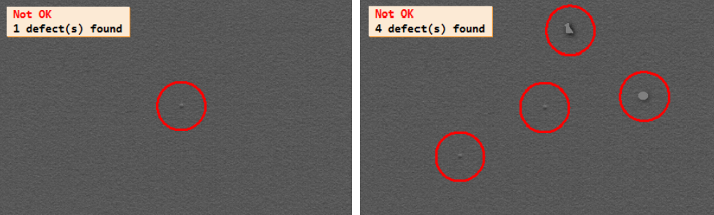
Frequency domain processing can also be used to deal with such subtle defects. The key of this routine is to use two low-pass filters and construct a band stop filter after subtraction (first pass the high contrast to let the medium and high frequency pass, then suppress the high frequency through Gaussian blur, and the final result is to let the medium frequency pass) to extract the defect component.

In addition, there is a routine using Fourier transform in Halcon: detect_mura_defects_texture.hdev

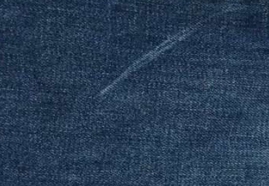
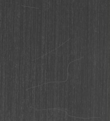
🐒 Detect scratches on cloth surface

*<Halcon Machine vision algorithm principle and programming practice 16-1
* Convert the test image into a single channel gray image
rgb1_to_gray (Image, ImageGray)

* 1.Create a Gaussian filter to filter the Fourier transformed image
gen_gauss_filter (GaussFilter, 3.0, 3.0, 0.0, 'none', 'rft', Width, Height)

* Color inversion of gray image
invert_image (ImageGray, ImageInvert)
* 2.Fourier transform the inverted image
rft_generic (ImageInvert, ImageFFT, 'to_freq', 'none', 'complex', Width)
* 3.Convolute the Fourier image and use the Gaussian filter created before as the convolution kernel
convol_fft (ImageFFT, GaussFilter, ImageConvol)
* 4.The convoluted Fourier image is restored to a spatial domain image. The abrupt part of the visible image is enhanced
rft_generic (ImageConvol, ImageFiltered, 'from_freq', 'n', 'real', Width)

* 5.Set the parameters of extracting lines to extract the lines with gray difference in the image
calculate_lines_gauss_parameters (17, [25,3], Sigma, Low, High)
lines_gauss (ImageFiltered, Lines, Sigma, Low, High, 'dark', 'true', 'gaussian', 'true')

🐎 Board scratch detection

*http://www.ihalcon.com/read-13031-1.html
dev_update_off ()
dev_close_window ()
read_image (Image, 'Defect detection and scratch extraction.jpg')
* 1.Color to grayscale image
count_channels (Image, Channels)
if (Channels == 3 or Channels == 4)
    rgb1_to_gray (Image, Image)
endif
get_image_size (Image, Width, Height)
dev_open_window_fit_size (0, 0, Width, Height, -1, -1, WindowHandle)
dev_display (Image)
* 2.Fourier transform background removal
fft_generic (Image, ImageFFT, 'to_freq', -1, 'sqrt', 'dc_center', 'complex')
gen_rectangle2 (Rectangle1, 308.5, 176.56, rad(-0), 179.4, 7.725)
gen_rectangle2 (Rectangle2, 306.955, 175, rad(-90), 180.765, 4.68)
union2 (Rectangle1, Rectangle2, UnionRectangle)
paint_region (UnionRectangle, ImageFFT, ImageResult, 0, 'fill')
fft_generic (ImageResult, ImageFFT1, 'from_freq', 1, 'sqrt', 'dc_center', 'byte')
* 3.Scratch extraction
threshold (ImageFFT1, Regions, 5, 240)
connection (Regions, ConnectedRegions)
select_shape (ConnectedRegions, SelectedRegions, 'area', 'and', 20, 99999)
union1 (SelectedRegions, RegionUnion)
dilation_rectangle1 (RegionUnion, RegionDilation, 5, 5)
connection (RegionDilation, ConnectedRegions1)
select_shape (ConnectedRegions1, SelectedRegions1, ['width','height'], 'and', [30,15], [150,100])
dilation_rectangle1 (SelectedRegions1, RegionDilation1, 11, 11)
union1 (RegionDilation1, RegionUnion1)
skeleton (RegionUnion1, Skeleton)
* 4.display
dev_set_color ('red')
dev_display (Image)
dev_display (Skeleton)

3.3 photometric stereo

In the industrial field, surface detection is a very wide application field. In halcon, three-dimensional surface detection is enhanced by using the enhanced photometric stereo vision method. The use of shadow can facilitate and quickly detect the notch or dent on the surface of the object. Using photometric stereo vision method, surface defects can be easily found in complex images.

• Applicable scenario: it is applicable to detect the concave convex features on metal materials.
  Detection principle:
  1. Through photo metric_ Stereo operator obtains surface gradient image, which can obtain surface gradient image and albedo image. You need to input multiple images obtained by lighting from different angles.
  2. Through derive_ vector_ The Gaussian (average) curvature image is obtained by the field operator, in which the surface gradient image obtained above needs to be input.
  Light source: photometric stereo method does not need special light source, only needs to shine from different angles.

Operator photometric_ Detailed explanation of stereo:

* Surface reconstruction using photometric stereo method
photometric_stereo (Images : HeightField, Gradient, Albedo : Slants, Tilts, ResultType, ReconstructionMethod, GenParamName, GenParamValue : )
* Images: Input image (4)
* HeightField: Return to the reconstructed height field
* Gradient: Returns the gradient field of the surface
* Albedo: Reflectivity of surface
* Slants: Included angle between light source and camera optical axis (schematic diagram below)
* Tilts: The included angle between the light projection of the light source and the principal axis of the measured object
* ResultType: Request result type (altitude field)/Gradient field/Reflectivity)
* ReconstructionMethod: Reconstruction method type
* GenParamName: General parameter name
* GenParamValue: General parameter setting

Operator derive_ vector_ Field details:

* Gradient field to mean curvature field
derivate_vector_field(VectorField : Result : Sigma, Component : )
* VectorField: Gradient field image
* Result: Returns the average curvature field image
* Sigma: Gaussian coefficient
* Component: Component calculation

3.3.1 preliminary photometric stereo method

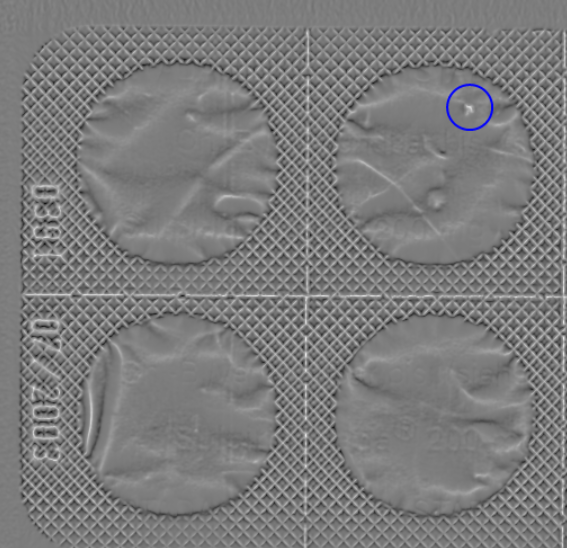
🐨 Detection of outer package damage of tablets

Halcon case: Method - photometric stereo method - inspect_blister_photometric_stereo.hdev

read_image (Images, './blister_back_0' + [1:4])
for I := 1 to 4 by 1
    select_obj (Images, ObjectSelected, I)
    *wait_seconds (0.1)
endfor

Tilts := [6.1,95.0,-176.1,-86.8]
Slants := [41.4,42.6,41.7,40.9]
* Photometric stereo
photometric_stereo (Images, HeightField, Gradient, Albedo, Slants, Tilts, 'all', 'poisson', [], [])
* Gradient field to mean curvature field
derivate_vector_field (Gradient, Result, 1, 'mean_curvature')
*scale_image_max (Result, ImageScaleMax)
* Seed growth
regiongrowing (Result, Regions, 1, 1, 0.01, 250)
select_shape (Regions, SelectedRegions, 'area', 'and', 16332.6, 28629.5)
shape_trans (SelectedRegions, RegionTrans, 'convex')
union1 (RegionTrans, RegionUnion)
erosion_circle (RegionUnion, RegionErosion, 3.5)
reduce_domain (Result, RegionErosion, ImageReduced)

* Find the absolute value of the image
abs_image (ImageReduced, ImageAbs)
threshold (ImageAbs, Regions1, 0.3, 0.5)
* display

In addition, the routine of photometric stereo method is as follows:

1. inspect_shampoo_label_photometric_stereo.hdev

2. Inspection_leather_photographic_stereo.hdev

Routine parsing reference: halcon -- Summary of common methods of defect detection (photometric stereo)

Poke little hand to help point out a free praise and attention, hey hey.

reference material:
1. WeChat official account: Machine Vision
2.https://www.cnblogs.com/xyf327/p/14872873.html
3.http://www.ihalcon.com/read-16432.html
4.https://blog.csdn.net/weixin_38566632/article/details/116377384
6.https://libaineu2004.blog.csdn.net/article/details/105366681
6.The strangulation tutorial of Fourier analysis (full version) was updated on June 6, 2014 - Zhihu (zhihu.com)；
7.Fourier transform of image
8.Photometric stereo