1, Access code
Get code method 1:
The complete code has been uploaded to my resources: [speech recognition] dial up speech recognition based on matlab GUI [including Matlab source code 1753]
Get code method 2:
By subscribing to the payment column of zijishenguang blog, private bloggers can obtain this code with payment vouchers.
remarks:
If you subscribe to the paid column of zijishenguang blog, you can get a code for free (valid for three days from the Subscription Date);
2, Introduction to DTMF
1 meaning
Dual Tone Multi Frequency DTMF (Dual Tone Multi Frequency) is composed of high-frequency group and low-frequency group, and the high-frequency group and low-frequency group each contain four frequencies. A high-frequency signal and a low-frequency signal are superimposed to form a combined signal, representing a number. DTMF signaling has 16 codes. DTMF signaling can be used to call the corresponding interphone.
Dual tone multifrequency signal (DTMF), a kind of user signaling between telephone and exchange in telephone system, is usually used to send the called number.
Before using DTMF signals, the telephone system uses a series of intermittent pulses to transmit the called number, which is called pulse dialing. Pulse dialing requires operators in the telecommunications bureau to manually complete long-distance connection.
Dual tone multifrequency signal was invented by Bell Labs. Its purpose is to automatically complete long-distance calls.
DTMF dialing keyboard is 4 × 4 matrix, each row represents a low frequency and each column represents a high frequency. Each press of a key sends a combination of high-frequency and low-frequency sinusoidal signals. For example, '1' is equivalent to 697 and 1209 Hertz (Hz). The switch can decode these frequency combinations and determine the corresponding keys.
The DTMF codec converts the keystroke or digital information into a two tone signal and sends it during encoding, and detects the existence of keystroke or digital information in the received DTMF signal during decoding. A DTMF signal is composed of audio signals of two frequencies superimposed. The frequencies of the two audio signals come from two pre allocated frequency groups: row frequency group or column frequency group. Each pair of such audio signals uniquely represents a number or symbol. There are usually 16 keys in the telephone, including 10 numeric keys 0 ~ 9 and 6 function keys *, #, a, B, C and D. According to the combination principle, there are generally 8 different single audio signals. Therefore, there are also 8 kinds of frequencies that can be used, so it is called multi frequency. Because it uses any combination of 2 out of 8 frequencies for coding, it is also called "2 out of 8" coding technology. According to CCITT's recommendations, 8 frequencies are adopted internationally, including 687Hz, 770Hz, 852Hz, 941Hz, 1209Hz, 1336Hz, 1477Hz and 1633Hz. 16 different combinations can be formed with these 8 frequencies to represent 16 different numbers or function keys. See Table 1 for specific combinations.
Tone detection is required in many applications, such as dual tone multi frequency signal (DTMF) decoding, call process (dial tone, busy tone, etc.) decoding, frequency response test (send a tone and read the result back at the same time). In the frequency response test, if the measurement is carried out within a certain frequency range, the obtained frequency response curve may contain rich information. For example, from the frequency response curve of the telephone line, we can know whether there is a load coil (inductance) on the line.
Although there are special IC s for the above applications, the cost of using software to realize the functions of these chips is much lower than that of using special chips. However, many embedded systems do not have the ability of continuous real-time FFT processing. At this time, Goertzel algorithm is suitable. This paper will discuss Goertzel basic algorithm and Goertzel optimization algorithm.
Using Goertzel's basic algorithm, the real and imaginary parts of the same frequency as the conventional discrete Fourier transform (DFT) or FFT can be obtained. If necessary, the amplitude and phase information can also be calculated from the real and imaginary parts of the frequency. Goertzel optimization algorithm is faster and simpler than Goertzel basic algorithm, but Goertzel optimization algorithm does not give the real and imaginary components of frequency, it can only give the relevant amplitude square. If the amplitude information is needed, it can be obtained by prescribing the result, but the phase information cannot be obtained by this method.
2 Goertzel basic algorithm
Goertzel basic algorithm is processed immediately after each sampling, and tone detection is performed once in each nth sampling. When using FFT algorithm, we need to process the samples in blocks, but this does not mean that we must process the data in blocks. The time of digital processing is very short, so if there is an interrupt for each sampling, these digital processing can be completed in the interrupt service program (ISR). Alternatively, if there is a sampling cache in the system, you can continue sampling and then batch processing.
Before actually running Goertzel algorithm, the following preliminary calculation must be carried out:
- Determine the sampling rate;
- Select the block size, i.e. N;
- Perform a cosine and sine calculation in advance;
- Calculate a coefficient in advance.
These calculations can be completed in advance and then hard coded into the program, so as to save RAM and ROM space, and can also be calculated dynamically.
3 select the appropriate sampling rate
In fact, the sampling rate may have been determined by the application itself. For example, 8kHz sampling rate is widely used in telecommunication applications, that is, 8000 samples per second. For another example, the operating frequency of analog-to-digital converter (or codec) may be determined by an external clock or external crystal oscillator that we cannot control.
However, if we can choose the sampling rate, we must follow Nyquist sampling theorem: the sampling rate is at least twice the maximum signal frequency. This is because if we want to detect multiple frequencies, using a higher sampling rate may get better results. Moreover, we all hope that there is an integer multiple relationship between the sampling rate and each frequency of interest.
4 block size setting
The block size n in Goertzel algorithm is similar to the number of points in the corresponding FFT, which controls the size of frequency resolution. For example, if the sampling rate is 8kHz and N is 100 samples, the frequency resolution is 80Hz.
This makes it possible for us to take n as high as possible in order to obtain the maximum frequency resolution. However, the larger the N, the more time it takes to detect each tone, because we have to wait until all the n samples are completed before we can start processing. For example, when the sampling rate is 8kHz, it takes 100ms to accumulate 800 samples. If you want to shorten the time of detecting tones, you must adjust the value of N appropriately.
Another factor affecting the selection of n is the relationship between sampling rate and target frequency. Ideally, the target frequency is within the midpoint of the corresponding frequency resolution, that is, we want the target frequency to be sample_ An integral multiple of the rate / N ratio. Fortunately, N in Goertzel algorithm is different from that in FFT, which does not have to be an integer power of 2.
5 pre calculated constant
After the sampling rate and block size are determined, the constants required for processing only need to be calculated through the following five simple calculations:
k = (Ntarget_freq)/sample_tate
w = (2π/N)*k
cosine = cos w
sine = sin w
coeff = 2 * cosine
Each sampling process requires three variables, which we call Q0 ', Q1' and Q2. Q1 is the Q0 value of the previous sampling process, and Q2 is the Q0 value before two sampling (or the value of Q1 before this sampling).
At the beginning of each sampling block, Q1 and Q2 must be initialized to 0. Each sample needs to be calculated according to the following three equations:
Q0 = coeff * Q1 - Q2 + sample
Q2 = Q1
Q1 = Q0
After N times of pre sampling calculation, the presence of tone can be detected.
real = (Q1 - Q2 * cosine)
imag = (Q2 * sine)
magnitude2 = real2 + imag2
At this time, it only needs a simple amplitude threshold test to judge whether there is a tone. After that, reset Q2 and Q1 to 0 and start the processing of the next block.
6 Goertzel optimization algorithm
Goertzel optimization algorithm requires less computation than Goertzel basic algorithm, but it is at the cost of losing phase information.
In Goertzel optimization algorithm, each sampling processing is exactly the same, but the processing result is different from Goertzel basic algorithm. In Goertzel's basic algorithm, it is usually necessary to calculate the real part and imaginary part of the signal, and then convert the calculation results of the real part and imaginary part into the corresponding amplitude square. In the optimized Goertzel algorithm, the real part and imaginary part do not need to be calculated, and the following formula is calculated directly:
magnitude2 = Q12 + Q22-Q1Q2coeff
3, Partial source code
function varargout = VoiceRecognition(varargin)
% VOICERECOGNITION MATLAB code for VoiceRecognition.fig
% VOICERECOGNITION, by itself, creates a new VOICERECOGNITION or raises the existing
% singleton*.
%
% H = VOICERECOGNITION returns the handle to a new VOICERECOGNITION or the handle to
% the existing singleton*.
%
% VOICERECOGNITION('CALLBACK',hObject,eventData,handles,...) calls the local
% function named CALLBACK in VOICERECOGNITION.M with the given input arguments.
%
% VOICERECOGNITION('Property','Value',...) creates a new VOICERECOGNITION or raises the
% existing singleton*. Starting from the left, property value pairs are
% applied to the GUI before VoiceRecognition_OpeningFcn gets called. An
% unrecognized property name or invalid value makes property application
% stop. All inputs are passed to VoiceRecognition_OpeningFcn via varargin.
%
% *See GUI Options on GUIDE's Tools menu. Choose "GUI allows only one
% instance to run (singleton)".
%
% See also: GUIDE, GUIDATA, GUIHANDLES
% Edit the above text to modify the response to help VoiceRecognition
% Last Modified by GUIDE v2.5 08-Apr-2020 19:08:03
% Begin initialization code - DO NOT EDIT
gui_Singleton = 1;
gui_State = struct('gui_Name', mfilename, ...
'gui_Singleton', gui_Singleton, ...
'gui_OpeningFcn', @VoiceRecognition_OpeningFcn, ...
'gui_OutputFcn', @VoiceRecognition_OutputFcn, ...
'gui_LayoutFcn', [] , ...
'gui_Callback', []);
if nargin && ischar(varargin{1})
gui_State.gui_Callback = str2func(varargin{1});
end
if nargout
[varargout{1:nargout}] = gui_mainfcn(gui_State, varargin{:});
else
gui_mainfcn(gui_State, varargin{:});
end
% End initialization code - DO NOT EDIT
%%
% --- Executes just before VoiceRecognition is made visible.
function VoiceRecognition_OpeningFcn(hObject, eventdata, handles, varargin)
% This function has no output args, see OutputFcn.
% hObject handle to figure
% eventdata reserved - to be defined in a future version of MATLAB
% handles structure with handles and user data (see GUIDATA)
% varargin command line arguments to VoiceRecognition (see VARARGIN)
% Choose default command line output for VoiceRecognition
handles.output = hObject;
% Update handles structure
guidata(hObject, handles);
% UIWAIT makes VoiceRecognition wait for user response (see UIRESUME)
% uiwait(handles.figure1);
%%
% --- Outputs from this function are returned to the command line.
function varargout = VoiceRecognition_OutputFcn(hObject, eventdata, handles)
% varargout cell array for returning output args (see VARARGOUT);
% hObject handle to figure
% eventdata reserved - to be defined in a future version of MATLAB
% handles structure with handles and user data (see GUIDATA)
% Get default command line output from handles structure
varargout{1} = handles.output;
%%
% --- Executes on button press in pushbutton2.
function pushbutton2_Callback(hObject, eventdata, handles)
% hObject handle to pushbutton2 (see GCBO)
% eventdata reserved - to be defined in a future version of MATLAB
% handles structure with handles and user data (see GUIDATA)
TextOut1 = 'Recording';
set( handles.edit1, 'String', TextOut1 ); % Display processing data in the interactive interface
myrecorder = audiorecorder(44100,16,1);
recordblocking(myrecorder,8);
recorder_array = getaudiodata(myrecorder);
recorder_array = recorder_array';
% pause(1);
audiowrite('Recording file.wav',recorder_array,44100);
TextOut2 = 'Recording complete';
set( handles.edit1, 'String', TextOut2 ); % Display processing data in the interactive interface
%%
% --- Executes on button press in pushbutton3.
function pushbutton4_Callback(hObject, eventdata, handles)
% hObject handle to pushbutton3 (see GCBO)
% eventdata reserved - to be defined in a future version of MATLAB
% handles structure with handles and user data (see GUIDATA)
% Initialization related parameters
load('recorder_filter.mat');%load Filter settings, bandpass 600-1600
bohao = [697,1209;697,1336;697,1477;770,1209;770,1336;770,1477;852 1209;852 1336;852 1477;941 1336];%From 1-9-0 Frequency of
[recorder,fs]=audioread('Generate audio file.wav');%Recording file
% sound(recorder,fs);
N = length(recorder);%Length of audio file
% figure(1);plot((1:N)/fs,recorder);
% Filter the recording
recorder = filter(recorder_filter,1,recorder);
recorder(abs(recorder)<0.001) = 0;
% Find short-term energy
wlen=200; inc=80; % The frame length and frame shift are given
win=hanning(wlen); % Haining window
X=enframe(recorder,win,inc)'; % Framing
fn=size(X,2); % Find the number of frames
time=(0:N-1)/fs; % Calculate the time scale of the signal
for i=1 : fn
u=X(:,i); % Take out a frame
u2=u.*u; % Find the energy
En(i)=sum(u2); % Summation of a frame
end
frameTime=frame2time(fn,wlen,inc,fs); % Find the time corresponding to each frame
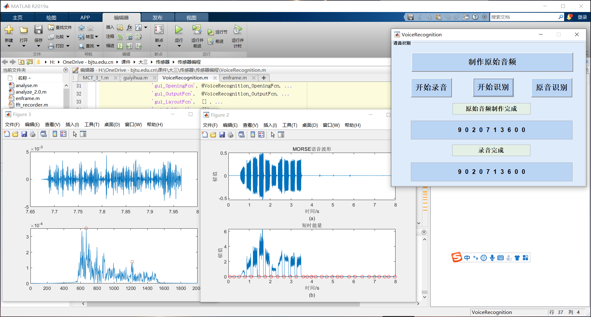
figure(2);
subplot 211; plot(time,recorder); % Draw the time waveform
title('MORSE Speech waveform');
ylabel('amplitude'); xlabel(['time/s' 10 '(a)']);
subplot 212; plot(frameTime,En) % Draw a short-term energy diagram
title('Short time energy');
ylabel('amplitude'); xlabel(['time/s' 10 '(b)']);
% By inverting the short-time energy,utilize findpeaks Function finding trough
En_reverse = [];
En_reverse = max(En)*3 - En;%Reverse
[minv,minl]=findpeaks(En_reverse,'minpeakdistance',100);%Find troughs with an interval of 100 frames
hold on;plot(frameTime(minl),En(minl),'o','color','r');hold off;
% The audio is segmented to obtain a separate single dial segment
En(En<0.00001) = 0;
target = En(minl);
point = [];
for i =1:length(minl)
point(i) = find(time==frameTime(minl(i)));
end
4, Operation results
5, matlab version and references
1 matlab version
2014a
2 references
[1] Han Jiqing, Zhang Lei, Zheng tieran Speech signal processing (3rd Edition) [M] Tsinghua University Press, 2019
[2] Liu ruobian Deep learning: Practice of speech recognition technology [M] Tsinghua University Press, 2019